 Cleve’s Corner: Cleve Moler on Mathematics and Computing
 The MATLAB Blog
 Guy on Simulink
 MATLAB Community
 Artificial Intelligence
 Developer Zone
 Stuart’s MATLAB Videos
 Behind the Headlines
 File Exchange Pick of the Week
 Hans on IoT
 Student Lounge
 MATLAB ユーザーコミュニティー
 Startups, Accelerators, & Entrepreneurs
 Autonomous Systems
 Quantitative Finance
 MATLAB Graphics and App Building
Symplectic Spacewar
This is the probably the first article ever written with the title "Symplectic Spacewar". If I Google that title today, including the double quotes to keep the two words together, I do not get any hits. But as soon as Google notices this post, I should be able to see at least one hit.
 And here is a photo, taken at the Vintage Computer Fair in 2006, of Steve and the PDP-1. The graphics display, an analog cathrode ray tube driven by the computer, can be seen over Steve's shoulder. The bank of sense switches is at the base of the console.
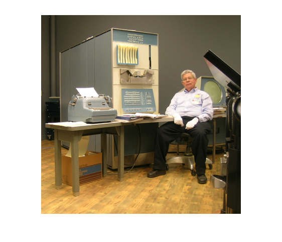 A terrific Java web applet, written by Barry and Brian Silverman and Vadim Gerasimov, provides a simulation of PDP-1 machine instructions running Spacewar. It is available here. Their README files explains how to use the keyboard in place of the sense switches. You should start by learning how to turn the spaceship and fire its rockets to avoid being dragged into the star and destroyed.
 Steve Russell certainly didn't know that his Spacewar was using a symplectic integrator. That term wasn't invented until years later. It is serendipity that the shortest machine language program has the best numerical properties.
Contents
Symplectic
Symplectic is an infrequently used mathematical term that describes objects joined together smoothly. It also has something to do with fish bones. For us, it is a fairly new class of numerical methods for solving certain special types of ordinary differential equations.Spacewar
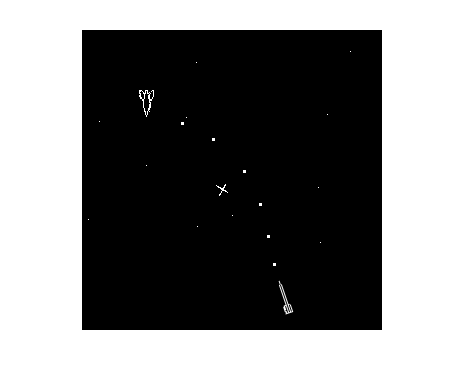
Spacewar is now generally recognized as the world's first video game. It was written by Steve "Slug" Russell and some of his buddies at MIT in 1962. Steve was a reseach assistant for Professor John McCarthy, who moved from MIT to Stanford in 1963. Steve came to California with McCarthy, bringing Spacewar with him. I met Steve then and played Spacewar a lot while I was a grad student at Stanford. Spacewar ran on the PDP-1, Digital Equipment Corporation's first computer. Two space ships, controlled by players using switches on the console, shoot space torpedoes at each other. The space ships and the torpedoes orbit around a central star. Here is a screen shot.X = imread('https://blogs.mathworks.com/images/cleve/Spacewar1.png');
imshow(X)
And here is a photo, taken at the Vintage Computer Fair in 2006, of Steve and the PDP-1. The graphics display, an analog cathrode ray tube driven by the computer, can be seen over Steve's shoulder. The bank of sense switches is at the base of the console.
X = imread('https://blogs.mathworks.com/images/cleve/Steve_Russell.png');
imshow(X)
A terrific Java web applet, written by Barry and Brian Silverman and Vadim Gerasimov, provides a simulation of PDP-1 machine instructions running Spacewar. It is available here. Their README files explains how to use the keyboard in place of the sense switches. You should start by learning how to turn the spaceship and fire its rockets to avoid being dragged into the star and destroyed.
Circle generator
The gravitational pull of the star causes the ships and torpedos to move in elliptical orbits, like the path of the torpedo in the screen shot. Steve's program needed to compute these trajectories. At the time, there was nothing like MATLAB. Programs were written in machine language, with each line of the program corresponding to a single machine instruction. I don't think there was any floating point arithmetic hardware; floating point was probably done in software. In any case, it was desirable to avoid evaluation of trig functions in the orbit calculations. The orbit-generating program would have looked something like this. x = 0
y = 32768
L: plot x y
load y
shift right 2
add x
store in x
change sign
shift right 2
add y
store in y
go to L
What does this program do? There are no trig functions, no square roots, no multiplications or divisions. Everything is done with shifts and additions. The initial value of y, which is $2^{15}$, serves as an overall scale factor. All the arithmetic involves a single integer register. The "shift right 2" command takes the contents of this register, divides it by $2^2$, and discards any remainder.
Notice that the current value of y is used to update x, then this new x is used to update y. This optimizes both instruction count and storage requirements because it is not necessary to save the current x to update y. But, as we shall see, this is also the key to the method's numerical stability.
Original
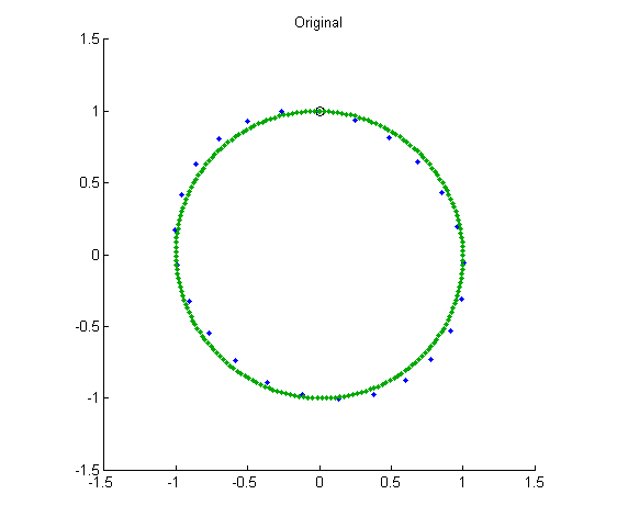
If the Spacewar orbit generator were written today in MATLAB, it would look something the following. There are two trajectories, with different step sizes. The blue trajectory has h = 1/4, corresponding to "shift right 2". The green trajectory has h = 1/32, corresponding to "shift right 5". We are no longer limited to integer values, so I have changed the scale factor from $2^{15}$ to $1$. The trajectories are not exact circles, but in one period they return to near the starting point. Notice, again, that the current y is used to update x and then the new x is used to update y.clf axis(1.5*[-1 1 -1 1]) axis square bg = 'blue'; for h = [1/4 1/32] x = 0; y = 1; line(x,y,'marker','o','color','k') for t = 0:h:2*pi line(x,y,'marker','.','color',bg) x = x + h*y; y = y - h*x; end bg = [0 2/3 0]; end title('Original')
Euler's method
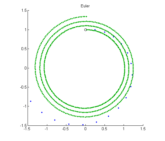
An exact circle would be generated by solving this system of ordinary differential equations. $$\dot{x}_1 = x_2$$ $$\dot{x}_2 = -x_1$$ This can be written in vectorized form as $$\dot{x} = A x$$ where $$A = \pmatrix{0 & 1 \cr -1 & 0}$$ The simplest method for computing an approximate numerical solution to this system, Euler's method, is $$x(t+h) = x(t) + h A x(t)$$ In the vectorized MATLAB code, all components of x are updated together. This causes the trajectories to spiral outward. Decreasing the step size decreases the spiraling rate, but does not eliminate it.clf axis(1.5*[-1 1 -1 1]) axis square bg = 'blue'; A = [0 1; -1 0]; for h = [1/4 1/32] x = [0 1]'; line(x(1),x(2),'marker','o','color','k') for t = 0:h:6*pi x = x + h*A*x; line(x(1),x(2),'marker','.','color',bg) end bg = [0 2/3 0]; end title('Euler')
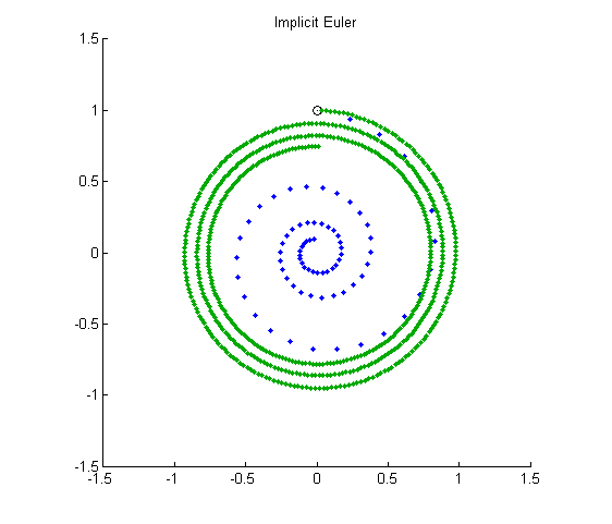
Implicit Euler
The implicit Euler method is intended to illustrate methods for stiff equations. This system is not stiff, but let's try implicit Euler anyway. Implicit methods usually involve the solution of a nonlinear algebraic system at each step, but here the algebraic system is linear, so backslash does the job. $$(I - h A) \ x(t+h) = x(t)$$ Again, all the components of the numerical solution are updated simultaneously. Now the trajectories spiral inward.clf axis(1.5*[-1 1 -1 1]) axis square bg = 'blue'; I = eye(2); A = [0 1; -1 0]; for h = [1/4 1/32] x = [0 1]'; line(x(1),x(2),'marker','o','color','k') for t = 0:h:6*pi x = (I - h*A)\x; line(x(1),x(2),'marker','.','color',bg) end bg = [0 2/3 0]; end title('Implicit Euler')
Eigenvalues
Eigenvalues are the key to understanding the behavior of these three circle generators. Let's start with the explicit Euler. The trajectories are given by $$ x(t+h) = E x(t) $$ where $$ E = I + h A = \pmatrix{1 & h \cr -h & 1} $$ The matrix $E$ is not symmetric. Its eigenvalues are complex, hence the circular behavior. The eigenvalues satisfy $$ \lambda_1 = \bar{\lambda}_2 $$ $$ \lambda_1 + \lambda_2 = \mbox{trace} (E) = 2 $$ $$ \lambda_1 \cdot \lambda_2 = \mbox{det} (E) = 1 + h^2 $$ The determinant is larger than 1 and the product of the eigenvalues is the determinant, so they must be outside the unit circle. The powers of the eigenvalues grow exponentially and hence so do the trajectories. We can reach this conclusion without actually finding the eigenvalues, even though that would be easy in this case. The implicit Euler matrix is the inverse transpose of the explicit matrix. $$ x(t+h) = E^{-T} x(t) $$ The eigenvalues of $E^{-T}$ are the reciprocals of the eigenvalues of $E$, so they are inside the unit circle. Their powers decay exponentially and hence so do the trajectories. Today, the spacewar circle generator would be called "semi-implicit". Explicit Euler's method is used for one component, and implicit Euler for the other. $$\pmatrix{1 & 0 \cr h & 1} x(t+h) = \pmatrix{1 & h \cr 0 & 1} x(t)$$ So $$x(t+h) = S x(h)$$ where $$S = \pmatrix{1 & 0 \cr h & 1}^{-1} \pmatrix{1 & h \cr 0 & 1} = \pmatrix{1 & h \cr -h & 1-h^2}$$ The eigenvalues satisfy $$ \lambda_1 + \lambda_2 = \mbox{trace} (S) = 2 - h^2 $$ $$ \lambda_1 \cdot \lambda_2 = \mbox{det} (S) = 1 $$ The key is the determinant. It is equal to 1, so we can conclude (without actually finding the eigenvalues) $$ |\lambda_1| = |\lambda_2| = 1$$ The powers $\lambda_1^n$ and $\lambda_2^n$ remain bounded for all $n$. It turns out that if we define $\theta$ by $$ \cos{\theta} = 1 - h^2/2 $$ then $$ \lambda_1^n = \bar{\lambda}_2^n = e^{i n \theta} $$ If, instead of an inverse power of 2, the step size $h$ happens to correspond to a value of $\theta$ that is $2 \pi / p$, where $p$ is an integer, then the spacewar circle produces only $p$ discrete points before it repeats itself. How close does our circle generator come to actually generating circles? The matrix $S$ is not symmetric. Its eigenvectors are not orthogonal. This can be used to show that the generator produces ellipses. As the step size $h$ gets smaller, the ellipses get closer to circles. It turns out that the aspect ratio of the ellipse, which is the ratio of its major axis to its minor axis, is equal to the condition number of the matrix of eigenvectors.Symplectic Integrators
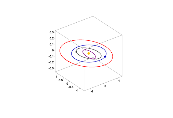
Symplectic methods for the numerical solution of ordinary differential equations apply to the class of equations derived from conserved quantities known as Hamiltonians. The components of the solution belong to two subsets, $p$ and $q$, and the Hamiltonian is a function of these two components, $H(p,q)$. The differential equations are $$\dot{p} = \frac{\partial H(p,q)}{\partial q}$$ $$\dot{q} = -\frac{\partial H(p,q)}{\partial p}$$ For our circle generator, $p$ and $q$ are the coordinates $x$ and $y$, and $H$ is one-half the square of the radius. $$H(x,y) = \textstyle{\frac{1}{2}}(x^2 + y^2)$$ Hamiltonian systems include models based on Newton's Second Law of Motion, $F = ma$. In this case $p$ is the position, $q$ is the velocity, and $H(p,q)$ is the energy. Symplectic methods are semi-implicit. They extend the idea of using the current value of $q$ to update $p$ and then using the new value of $p$ to update $q$. This makes it possible to conserve the value of $H(p,q)$, to within the order of accuracy of the method. The spacewar circle generator is a first order symplectic method. The radius is constant, to within an accuracy proportional to the step size $h$. For other examples of symplectic methods, including the n-body problem of orbital mechanics, see the Orbits chapter and the orbits.m program of Experiments with MATLAB. Here is a screen shot showing the inner planets of the solar system.X = imread('https://blogs.mathworks.com/images/cleve/solar2.png');
imshow(X)
Steve Russell certainly didn't know that his Spacewar was using a symplectic integrator. That term wasn't invented until years later. It is serendipity that the shortest machine language program has the best numerical properties.
References
[1] http://en.wikipedia.org/wiki/Spacewar!, Wikipedia article on Spacewar. [2] http://en.wikipedia.org/wiki/File:Steve_Russell_and_PDP-1.png, Steve Russell and the Computer History Museum's PDP-1 at the Vintage Computer Fair 2006.- Category:
- Matrices


Comments
To leave a comment, please click here to sign in to your MathWorks Account or create a new one.