 Cleve’s Corner: Cleve Moler on Mathematics and Computing
 The MATLAB Blog
 Guy on Simulink
 MATLAB Community
 Artificial Intelligence
 Developer Zone
 Stuart’s MATLAB Videos
 Behind the Headlines
 File Exchange Pick of the Week
 Hans on IoT
 Student Lounge
 MATLAB ユーザーコミュニティー
 Startups, Accelerators, & Entrepreneurs
 Autonomous Systems
 Quantitative Finance
 MATLAB Graphics and App Building
Further Twists of the Moebius Strip
The equations generating a surf plot of the Moebius strip can be parameterized and the parameters allowed to take on expanded values. The results are a family of surfaces that I have been displaying for as long as I have had computer graphics available.
Contents
Parametrized Moebius Strip
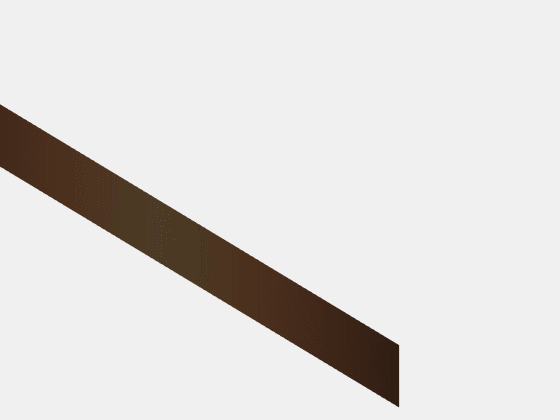
The animation shows the formation of a classic Moebius strip. Start with a long, thin rectangular strip of material. Bend it into a cylinder. Give the two ends a half twist. Then join them together. The result is a surface with only one side and one boundary. One could traverse the entire length of the surface and return to the starting point without ever crossing the edge.
I am going to investigate the effect of three free parameters:
- $c$: curvature of the cylinder.
- $w$: width of the strip.
- $k$: number of half twists.
These parameters appear in a mapping of variables $s$ and $t$ from the square $-1 <= s,t <= 1$ to a generalized Moebius strip in 3D.
$$ r = (1-w) + w \ s \ \sin{(k \pi t/2)} $$
$$ x = r \ \sin{(c \pi t)}/c $$
$$ y = r \ (1 - (1-\cos{(c\pi t))}/c) $$
$$ z = w \ s \ \cos{(k \pi t/2)} $$
Here is the code. The singularity at $c = 0$ can be avoided by using c = eps.
type moebius
function [x,y,z,t] = moebius(c,w,k)
% [x,y,z,t] = moebius(c,w,k)
% [x,y,z] = surface of moebius strip, use t for color
% c = curvature, 0 = flat, 1 = cylinder.
% w = width of strip
% k = number of half twists
    if c == 0
        c = eps;
    end
    m = 8;
    n = 128;
    [s,t] = meshgrid(-1:2/m:1, -1:2/n:1);
    r = (1-w) + w*s.*sin(k/2*pi*t);
    x = r.*sin(c*pi*t)/c;
    y = r.*(1 - (1-cos(c*pi*t))/c);
    z = w*s.*cos(k/2*pi*t);
end
The animation begins with a flat, untwisted strip of width 1/4, that is
$$ c = 0, \ w = 1/4, \ k = 0 $$
The classic Moebius strip is reached with
$$ c = 1, \ w = 1/4, \ k = 1 $$
The final portion of the animation simply changes the viewpoint, not the parameters.
Parula
Let's play with colormaps. I'll look at the classic Moebius strip and make the default MATLAB colormap periodic by appending a reversed copy. I think this looks pretty nice.
map = [parula(256); flipud(parula(256))];

HSV
The Hue-Saturation-Value color map has received a lot of criticism in MathWorks blogs recently, but it works nicely in this situation. This figure has $k = 4$, so there are two full twists. That's very hard to see from this view. The colors help, but it's important to be able to rotate the view, which we can't do easily in this blog.

TripleTwist
Here is the one with three half twists. Like the classic Moebius strip, this has only one side. I've grown quite fond of this guy, so I'll show two views. The HSV color map, with its six colors, works well.


IEEE Computer, 1988
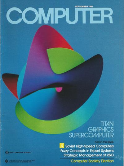
Source: IEEE
I have written in this blog about the glorious marriage between MATLAB and the Dore graphics system on the ill-fated Ardent Titan computer almost 30 years ago. I somehow generated this image using MATLAB, Dore, these parametrized Moebius equations and the Titan graphics hardware in 1988. This was fancy stuff back then. The editors of IEEE Computer were really excited about this cover.
I've never been able to reproduce it. I don't know what the parameters were.
Kermit Sigmon
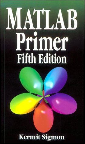
Kermit Sigmon was a professor at the University of Florida. He was an excellent teacher and writer. He wrote a short MATLAB Primer that was enormously popular and widely distributed in the early days of the web. It went through several editions and was translated into a couple of other languages.
For the most part, people had free copies of the MATLAB Primer without fancy covers. But CRC Press obtained the rights to produce a reasonably priced bound paperback copy which featured a cover with $k = 5$.
Kermit passed away in 1997 and Tim Davis took over the job of editing the Primer. He generated more elaborate graphics for his covers.


See Also
-

Rubik's Cube
Blogs


Comments
To leave a comment, please click here to sign in to your MathWorks Account or create a new one.