Loren on the Art of MATLAB

Contents

What's your problem! ?

Whenever I have a question about MATLAB that I can't figure out from the help or the doc, I only need to stick my head out of my office and ask my neighbor. Sometimes I wonder how I would get answers to my most challenging how-do-I questions if I were an isolated MATLAB user tucked away in a lab. I guess the chances are I would get them from the same source, but the medium would be via the MATLAB newsgroup (comp.soft-sys.matlab).

When I was new to MATLAB I would browse the newsgroup to learn. I found that learning from other people's questions was even more powerful than learning from their mistakes. As my knowledge of MATLAB has improved, I browse to get an insight into the usecases and usability problems in my subject area and try to help out if I can. There aren't many posts on computational geometry, but I have clicked on quite a few griddata subject lines and I was able to learn that for some users, griddata didn't quite "click". Now this wasn't because they were slow; it was because griddata was slow or deficient in some respect.

Despite its shortcomings, griddata is fairly popular, but it does trip up users from time to time. A new user can make a quick pass through the help example and they are up and running. They use it to interpolate their own data, get good results, and they are hooked. In fact, it may work so well in black-box mode that users don't concern themselves about the internals; that is, until it starts returning NaNs, or the interpolated surface looks bad close to the boundary, or maybe it looks bad overall. Then there's the user who fully understands what's going on inside the black box, but lacks the functionality to do the job efficiently. This user shares my frustrations; the black box is too confined and needs to be reusable and flexible so it can be applied to general interpolation scenarios.

griddata Produces "Funny" Results

griddata is useful, but it's not magic. You cannot throw in any old data and expect to get back a nice looking smooth surface like peaks. Like everything else in MATLAB it doesn't work like that. Sometimes our lack of understanding of what goes on in the inside distorts our perception of reality and our hopes to get lucky become artificially elevated. It's tempting to go down the path of diagnosing unexpected results from griddata, but I will have to leave that battle for another day. Besides, if you are reading this blog you are probably a savvy MATLAB user who is already aware of the usual pitfalls. But, I would like to provide one tip; if 2D scattered data interpolation produces unexpected results, create a Delaunay triangulation of the (x, y) locations and plot the triangulation. Ideally we would like to see triangles that are close to equilateral. If you see sliver shaped triangles then you cannot expect to get good results in that neighborhood. This example shows what I mean. I will use two new features from R2009a; DelaunayTri and TriScatteredInterp, but you can use the functions delaunay and griddata if you are running an earlier version.

I will create a distribution of points (red stars) that would produce concave boundaries if we were to join them like a dot-to-dot puzzle. I will then create a Delaunay triangulation from these points and plot it (blue triangles).

t= 0.4*pi:0.02:0.6*pi;
x1 = cos(t)';
y1 = sin(t)'-1.02;
x2 = x1;
y2 = y1*(-1);
x3 = linspace(-0.3,0.3,16)';
y3 = zeros(16,1);
x = [x1;x2;x3];
y = [y1;y2;y3];
dt = DelaunayTri(x,y);
plot(x,y, '*r')
axis equal
hold on
triplot(dt)
plot(x1,y1,'-r')
plot(x2,y2,'-r')
hold off

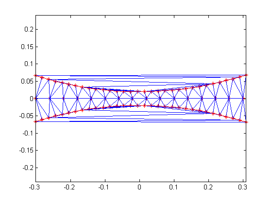
The triangles within the red boundaries are relatively well shaped; they are constructed from points that are in close proximity. We would expect the interpolation to work well in this region. Outside the red boundary, the triangles are sliver-like and connect points that are remote from each other. We do not have sufficient sampling in here to accurately capture the surface; we would expect the results to be poor in these regions.

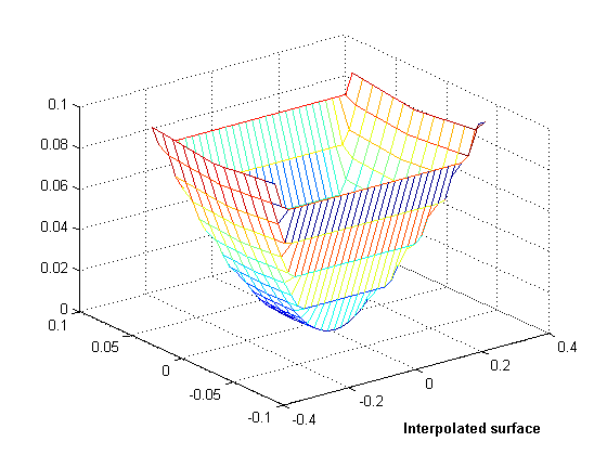
Let's see how the interpolation would look if we lifted the points to the surface of a paraboloid.

z = x.^2 + y.^2;
F = TriScatteredInterp(x,y,z);
[xi,yi] = meshgrid(-0.3:.02:0.3, -0.0688:0.01:0.0688);
zi = F(xi,yi);
mesh(xi,yi,zi)
xlabel('Interpolated surface', 'fontweight','b');

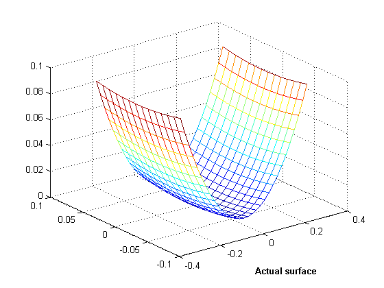
Now let's see what the actual surface looks like in this domain.

zi = xi.^2 + yi.^2;
mesh(xi,yi,zi)
xlabel('Actual surface', 'fontweight','b');

OK, you get the idea. You can see the parts of the interpolated surface that correspond to the sliver triangles. In 3D, visual inspection of the triangulation gets a bit trickier, but looking at the point distribution can often help illustrate potential problems.

Scattered Data Interpolation in the Real-World

Have you ever taken a vacation overseas and experienced the per-transaction exchange-rate penalty for credit card purchases? Oh yeah, you're on your way out the door of the gift shop with your bag of goodies, you realize you forgot someone and . . . . catchinggg catchinggg; you're hit with the exchange rate penalty again. But hey, it's a vacation, forget it. Besides, I'm not Mr Savvy Traveler. Now when you're back at work in front of MATLAB, per-transaction penalties have a completely different meaning. We have to be savvy to avoid them, but in reality we would simply prefer not to pay them.

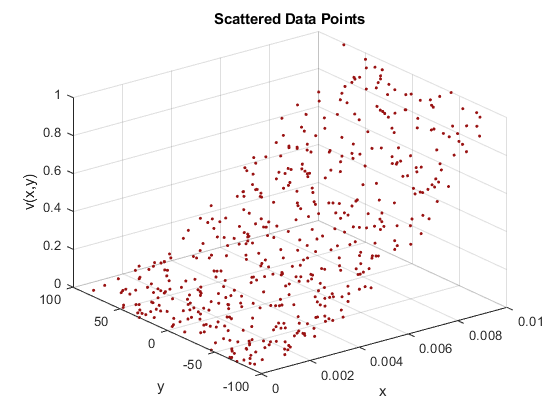
The scattered data interpolation tools in MATLAB are very useful for analyzing scientific data. When we collect sample-data from measurements, we often leverage the same equipment to gather various metrics of interest and sample over a period of time. Collecting weather data is a good example. We typically collect temperature, rainfall, and snowfall etc, at fixed locations across the country and we do this continuously. When we import this data into MATLAB we get to do the interesting part – analyze it. In this scenario we could use interpolation to compute weather data at any (longitude, latitude) location in the country. Assuming we have access to weather archives we could also make historical comparisons. For example, we could compute the total rainfall at (longitude, latitude) for years 2008, 2007, 2006 etc, and likewise we could do the same for total snowfall. If we were to use griddata to perform the interpolation, then catchinggg catchinggg, we would pay the unnecessary overhead of computing the underlying Delaunay triangulation each time a query is evaluated.

For example, suppose we have the following annual rainfall data for 2006-2008:

     (xlon, ylat, annualRainfall06)
     (xlon, ylat, annualRainfall07)
     (xlon, ylat, annualRainfall08)

xlon, ylat, and annualRainfall0* are vectors that represent the sample locations and the corresponding annual rainfall at these locations. We can use griddata to query by interpolation the annual rainfall zq at location (xq, yq).

     zq06 = griddata(xlon, ylat, annualRainfall06, xq, yq)
     zq07 = griddata(xlon, ylat, annualRainfall07, xq, yq)
     zq08 = griddata(xlon, ylat, annualRainfall08, xq, yq)

Note that a Delaunay triangulation of the points (xlon, ylat) is computed each time the interpolation is evaluated at (xq, yq). The same triangulation could have been reused for the 07 and 08 queries, since we only changed the values at each location. In this little illustrative example the penalty may not be significant because the number of samples is likely to be in the hundreds or less. However, when we interpolate large data sets this represents a serious transaction penalty. TriScatteredInterp, the new scattered data interpolation tool released in R2009a, allows us to avoid this overhead. We can use it to construct the underlying triangulation once and make repeated low-cost queries. In addition, for fixed sample locations the sample values and the interpolation method can be changed independently without re-triangulation. Repeating the previous illustration using TriScatteredInterp we would get the following:

     F = TriScatteredInterp(xlon, ylat, annualRainfall06)
     zq06 = F(xq, yq)
     F.V = annualRainfall07;
     zq07 = F(xq, yq)
     F.V = annualRainfall08;
     zq08 = F(xq, yq)

We can also change the interpolation method on-the-fly; this switches to the new Natural Neighbor interpolation method.

     F.Method = 'natural';

Again, no transaction penalty for switching the method. To evaluate using natural neighbor interpolation we do the following:

     zq08 = F(xq, yq)

As you can see, the interpolant works like a function handle making the calling syntax more intuitive.

What's the Bottom Line?

The new scattered data interpolation function, TriScatteredInterp, allows you to interpolate large data sets very efficiently. Because the triangulation is cached within the black-box (the interpolant) you do not need to pay the overhead of recomputing the triangulation each time you evaluate, change the interpolation method, or change the values at the sample locations.

What's more, as in the case of DelaunayTri, this interpolation tool uses the CGAL Delaunay triangulations which are robust against numerical problems. The triangulation algorithms are also faster and more memory efficient. So if you use MATLAB to interpolate large scattered data sets, this is great news for you.

The other bonus feature is the availability of the Natural Neighbor interpolation method – not be confused with Nearest Neighbor interpolation. Natural neighbor interpolation is a triangulation-based method that has an area-of-influence weighting associated with each sample point. It is widely used in the area of geostatistics because it is C1 continuous (except at the sample locations) and it performs well in both clustered and sparse data locations.

For more information on this feature and the new computational geometry features shipped in R2009a check out the overview video, and Delaunay triangulation demo, or follow these links to the documentation

Feedback

If you use MATLAB to perform scattered data interpolation, let me know what you think here. It's the feedback from users like you that prompts us to provide enhancements that are relevant to you.

Get the MATLAB code

Published with MATLAB® 7.8