
Table of ContentsLots of Code, Lots of Places Shared Files Code Reproducibility and Reuse Sites that Host MATLAB Interoperability with Other Languages Resources ConclusionsThere are lots of ways to... read more >>

Note
Loren on the Art of MATLAB has been archived and will not be updated.
Table of ContentsLots of Code, Lots of Places Shared Files Code Reproducibility and Reuse Sites that Host MATLAB Interoperability with Other Languages Resources ConclusionsThere are lots of ways to... read more >>

Before the pandemic (actually a couple of years before), as I was trying to find a super easy way to show the power of a pre-trained network in MATLAB, I made this example from my desk in the office.... read more >>


A mind-bending tale of adventure. A mildly distasteful yarn.Today's guest blogger is Rob Holt, who works at MathWorks in Natick, Massachusetts.Rob currently serves as the Manager for Biological... read more >>
Today's post is brought to you from Peter Perkins, a member of the MathWorks development team.Having worked on some of MATLAB's time and date functions, people at The MathWorks sometimes ask me... read more >>
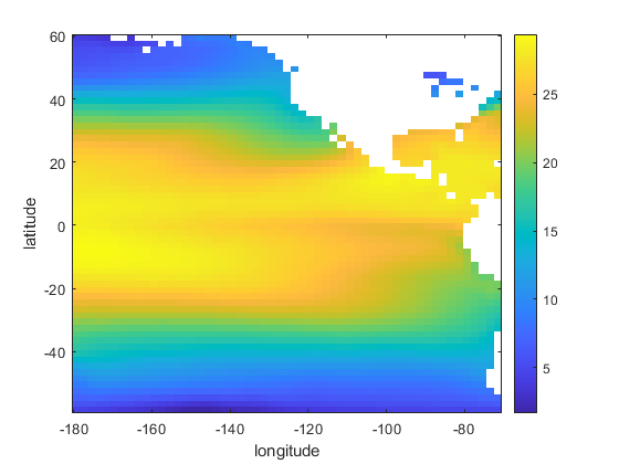
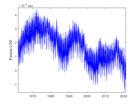
Today our guest blogger is Lisa Kempler, who works at MathWorks in Natick, Massachusetts. Lisa supports researchers and educators, frequently geoscientists, helping them build and host the tools that... read more >>
In a recent post, I talked about for-loops in MATLAB and how to optimize their use knowing how MATLAB stores arrays in memory. Today I want to talk about getting ready for parallel computation,... read more >>
Have you ever looked at code where you are calling a function with many arguments, many of which are strings, and find it hard to see what's going on? I know I have. And perhaps you too. In release... read more >>
Today I'd like to welcome a guest blogger, Mike Croucher, who recently joined MathWorks as a Customer Success Engineer after a long career spent supporting academic computational research.Table of... read more >>
I was talking to my long-time colleague, Mike Croucher, who joined MathWorks team recently (yay!). About a bunch of interesting topics, some of which could be good fodder for a blog post. Today I... read more >>

Today's guest blogger is Mary Fenelon, who is the product marketing manager for Optimization and Math here at MathWorks. In today's post she describes how using the new paged matrix functions can... read more >>
These postings are the author's and don't necessarily represent the opinions of MathWorks.