 Cleve’s Corner: Cleve Moler on Mathematics and Computing
 The MATLAB Blog
 Guy on Simulink
 MATLAB Community
 Artificial Intelligence
 Developer Zone
 Stuart’s MATLAB Videos
 Behind the Headlines
 File Exchange Pick of the Week
 Hans on IoT
 Student Lounge
 MATLAB ユーザーコミュニティー
 Startups, Accelerators, & Entrepreneurs
 Autonomous Systems
 Quantitative Finance
 MATLAB Graphics and App Building

Sean's pick this week is the collection of artistic images submitted by Jenny Bosten in the ongoing MATLAB Mini Hack.The mini hack is one of a few contests running to celebrate 20 years of MATLAB... read more >>
Convert Deep Learning Models between PyTorch, TensorFlow, and MATLAB
Three favorites from TIME Magazine’s “Best Innovations of 2023”
An interview with MATLAB playground: Build your IoT Analysis and Plots for ThingSpeak
MathWorks Training: Aligning development goals and team skills to enhance startup success
Sean's pick this week is the collection of artistic images submitted by Jenny Bosten in the ongoing MATLAB Mini Hack.The mini hack is one of a few contests running to celebrate 20 years of MATLAB... read more >>

Sean's pick this week is KronProd by Matt J.BackgroundThis one is old and very dear to my heart. Some time in the 2009 era, as I was starting grad school, I needed help calculating subpixel... read more >>
Today's post is by Lama Itani, who is part of the MathWorks Academic Engineering Team.
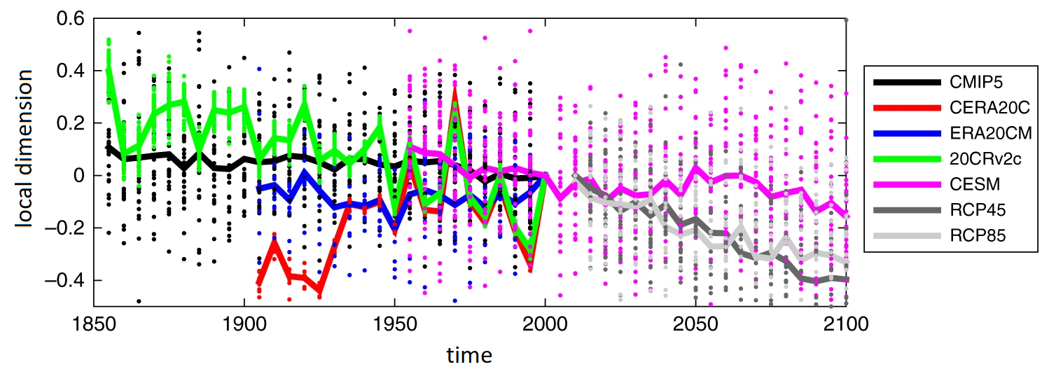
This week's Pick is Attractor Local Dimension and Local Persistence computation by Davide Faranda. This code... read more >>
Back in R2016b, we introduced tall arrays to facilitate, among other things, processing arbitrarily large datasets. This works nicely for tables or timetables, for example, and works in conjunction... read more >>
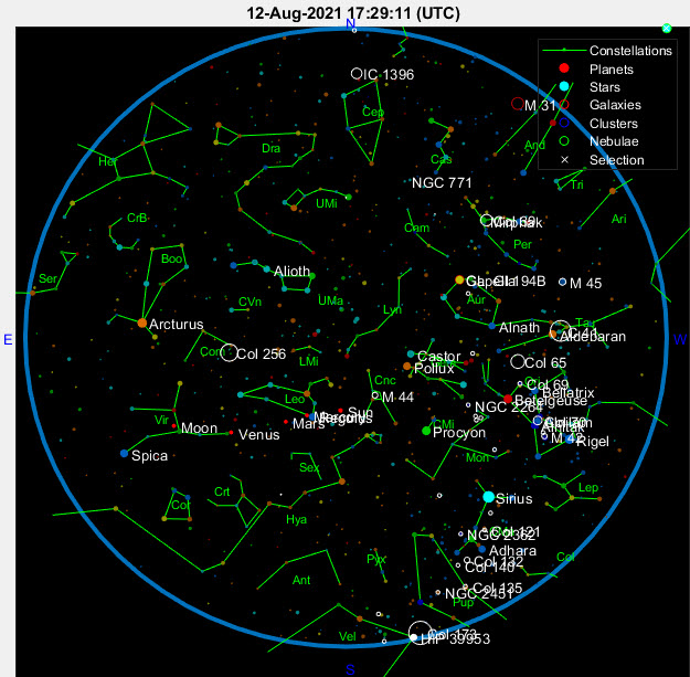
Will's pick this week is skychart by Emmanuel Farhi. This submission leverages object-oriented programming to plot celestial objects visible to a ground-based observer. Create an object, define... read more >>

Sean's pick this week is m2uml by per isakson. Table of Contents m2uml MATLAB's Class Diagram Viewer in R2021a Comments m2uml Have you ever had (or inherited!) a lot of classes... read more >>
Jiro's Pick this week is Unit Circle - Sine and Cosine Functions by Michal Blaho.Concepts become easier to understand when they can be visualized and explored by students. Back when I first learned... read more >>

Jiro's Pick this week is Import Explorer for tables by Jan Studnicka.When importing data as a table, you can use detectImportOptions to customize how you bring in your data. You can choose to import... read more >>
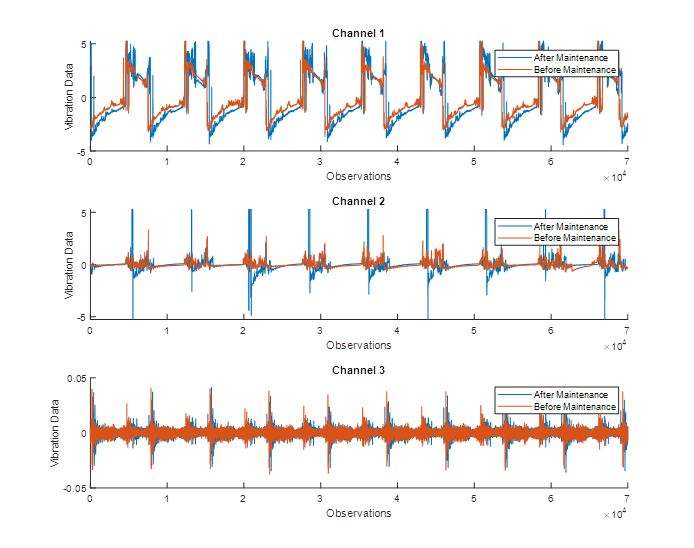
Rachel is the product manager for predictive maintenance at MathWorks. Rachel's pick this week is Industrial Machinery Anomaly Detection using an Autoencoder which she submitted! Today's... read more >>
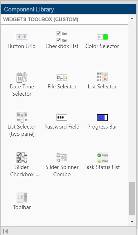
Sean's pick this week is Widgets Toolbox by Robyn Jackey. Contents Instagram... read more >>
These postings are the author's and don't necessarily represent the opinions of MathWorks.