
Did I just get a different answer?
As part of any well designed Model Based Design work-flow, you need to ensure that you get the expected results from your simulation. You might want to evaluate the effect of a change to the model, or just need to validate that your results are consistent between normal mode simulation and running the generated code.
To illustrate this idea, I will compare two signals generated from two slightly different implementations of the van der Pol equations. To keep this post simple, I will focus only on the state x2.
open_system('vdp_1')
open_system('vdp_2')
[t1,xout1] = sim('vdp_1');
[t2,xout2] = sim('vdp_2');
x1 = xout1(:,2);
x2 = xout2(:,2);
Quick test for equality
Do a quick test for equality between variables using isequal.
isequal(x1,x2)
ans =
     0
This gives you a fast way to cycle through tons of data and turn up the subset that requires further investigation.
For a sanity check, I think it is natural to plot the data to see if the difference is visible.
plot(t1,x1,t2,x2)
legend('Sim1','Sim2')
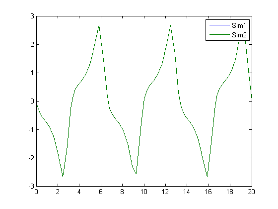
This is actually rarely helpful for small differences in signals. In this case, the green line is on top of the blue line, so they must be the same, right? Well, they must be the same at least to the resolution of my monitor. Depending on the reason you are comparing these signals, you might stop here, but if you need more precision, how about looking at the difference?
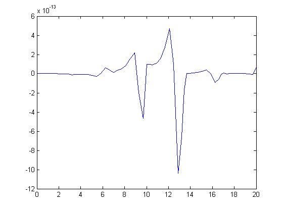
plot(t1,x1-x2)
Computing the Absolute Difference
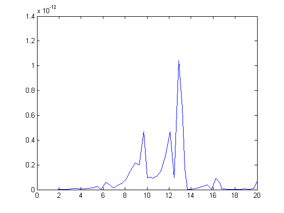
If signals are periodic, and the error is cumulative, the difference will generally also be periodic. I am often trying to evaluate if the difference is growing in magnitude or shrinking. I usually look at the absolute difference between signals.
x_diff = abs(x1-x2);
plot(t1,x_diff)
If you want a difference measure, you could imagine that your solution is a vector in a high dimensional vector space. I imagine the difference between the solutions to be the magnitude of the difference. To compute this, you might use the norm
nx = norm(x1-x2)
nx =
  1.5108e-012
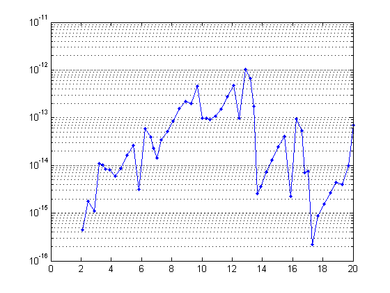
Because I often see a wide range of differences in signals, I think it is better to use a logarithmic scale in the plot. When differences enter into a system on the order of eps, and grow larger, the logarithmic scale will help draw attention to the small magnitude differences as much as the larger magnitude differences.
semilogy(t1,x_diff,'.-')
set(gca,'YGrid','on')
Now it's your turn
When do you compare signals? How do you do it? Leave a comment here and share your technique.


Comments
To leave a comment, please click here to sign in to your MathWorks Account or create a new one.