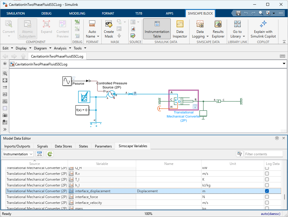
Did you know that starting in R2024a, it is possible to log Simscape variables like if they were Simulink signals?Let's see how that works.The ProblemHere is a pattern I often see in Simscape models.... read more >>

Did you know that starting in R2024a, it is possible to log Simscape variables like if they were Simulink signals?Let's see how that works.The ProblemHere is a pattern I often see in Simscape models.... read more >>
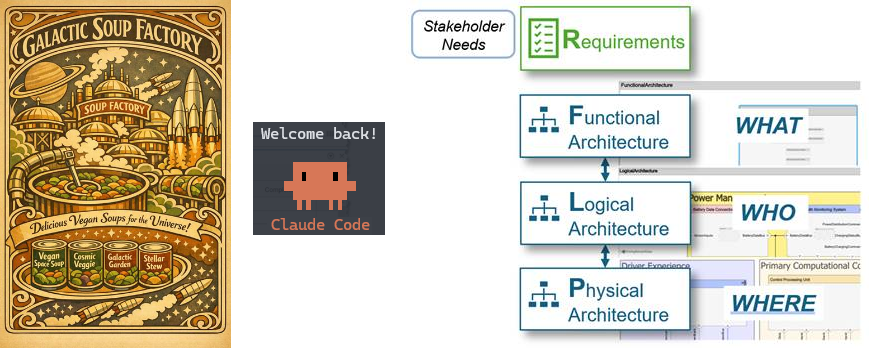
Today I am happy to welcome Sarah Dagen from MathWorks Consulting Services to talk about her experience with coding agents for Model-Based Systems Engineering..Like many of you, I’ve been exploring... read more >>
MATLAB R2026a is available, let's see what's new in the Simulink world.New Context MenuThis one cannot be missed! We decided to modernize our right-click menu.Here is what it looks like when you... read more >>

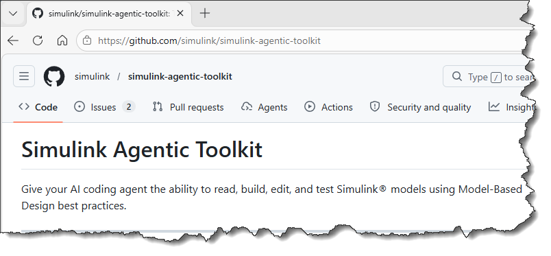
After the MATLAB Agentic Toolkit debuted last week, we are very happy to release the Simulink Agentic Toolkit on GitHub today.SetupTo get started, go through the README.md and GETTING_STARTED.md. You... read more >>
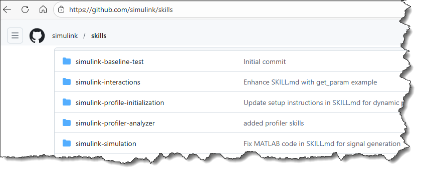
Update: The Simulink Agentic Toolkit is now available. I recommend installing the toolkit when interacting twith Simulink through an AI agent. Skills in this repository are complementary and should... read more >>
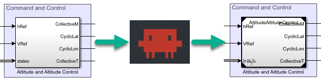
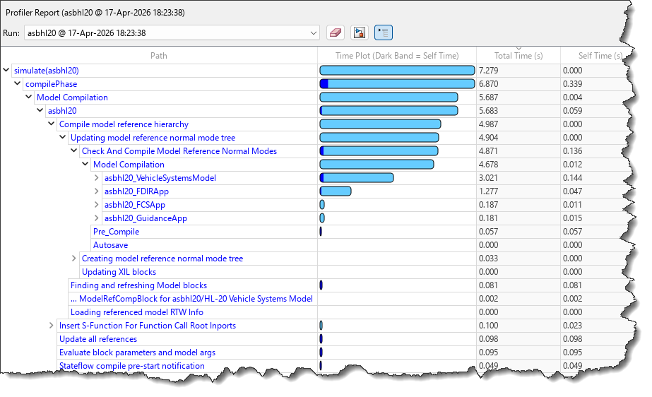
Once you start using those AI agents, it's hard to stop!In today's post, I used Amp, an AI coding agent made by Sourcegraph and similar to Claude Code, to do one of the tasks I help Simulink users... read more >>
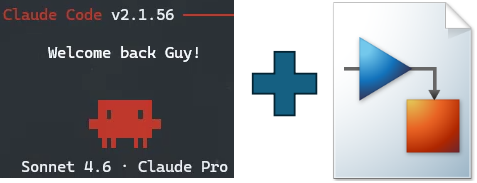
This week, I am going one step further in my exploration of AI agents and how they can help Simulink workflows. In previous posts, I went through the basics of connecting GitHub Copilot with the... read more >>
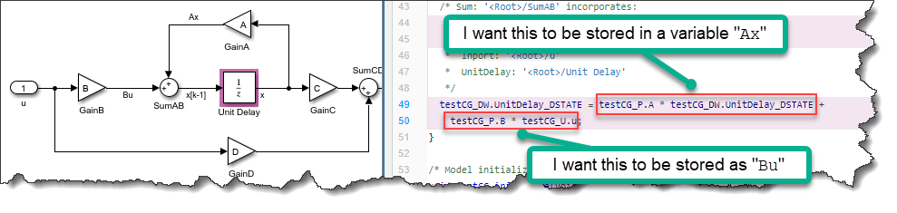
One of the key benefits of Simulink is that you can generate C/C++ code from the model using Simulink Coder and Embedded Coder.However, I have to admit, looking at the code generated from Simulink... read more >>

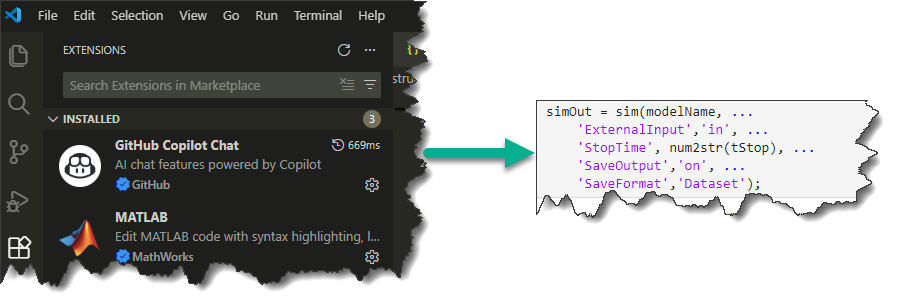
In my previous post, I went through the basics of using GitHub Copilot and the MATLAB MCP Server to generate MATLAB code that can simulate a Simulink. While the AI-generated code simulated the... read more >>
Today I am continuing my exploration in the world of AI coding assistants and how they can help with Simulink. The topic for this post: The MATLAB MCP Server.MATLAB MCP ServerMathWorks recently... read more >>
These postings are the author's and don't necessarily represent the opinions of MathWorks.