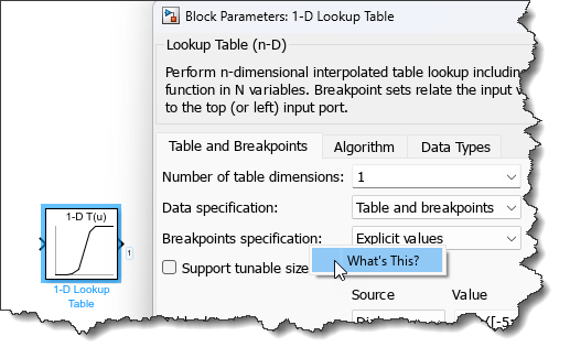
In my previous post, I introduced MATLAB Copilot and the Simulink Copilot Beta. Today, I continue my exploration into the world of AI assistants and how they can help in a Simulink context.What... read more >>

In my previous post, I introduced MATLAB Copilot and the Simulink Copilot Beta. Today, I continue my exploration into the world of AI assistants and how they can help in a Simulink context.What... read more >>

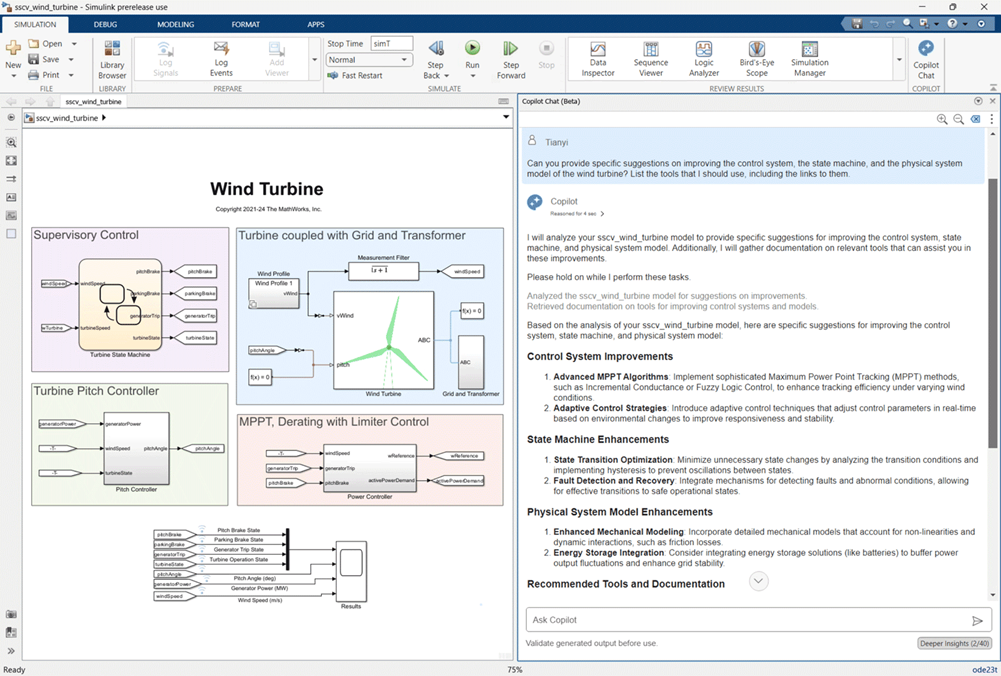
I recently decided to investigate different AI coding assistant technologies and see how they can help with Simulink. This led me into a series of blog posts that I plan to publish in the next few... read more >>
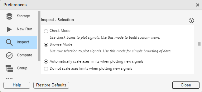
I receive and debug Simulink models all day every day. This means that I often need to log many signals and inspect them to understand what the model is doing.For that, I like using the Simulation... read more >>

Today I want to share a simple tip to interact with data logged from a Simulink modelThe ProblemLet's take this simple model that logs 3 signals with different sample times:After simulating, it is... read more >>
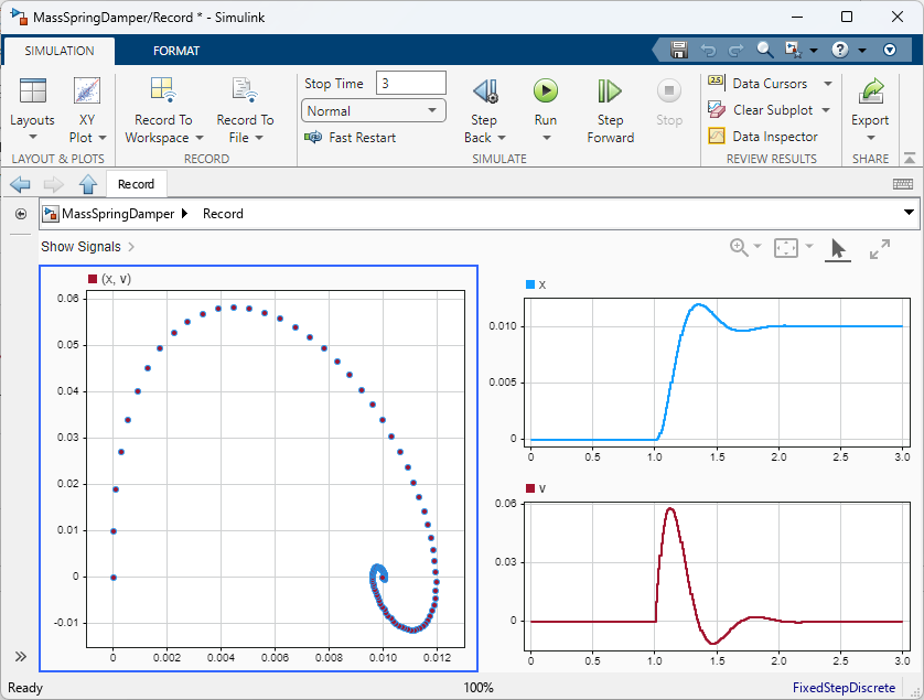
Today I want to talk about two relatively new blocks: Record and Playback.Record BlockLet's start with this simple example where I connect two signals to the Record block:mdl =... read more >>
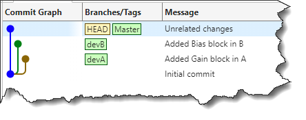
This post is targeted at users developing Simulink models under Git source control, but who are not necessarily using the MATLAB source control integration.I personally work in MATLAB and Simulink... read more >>
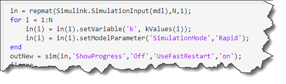
Here is another frequently viewed MATLAB Answers post:Set simulation time and fixed step size for a Simulink model from the command lineWhile this question asks specifically about stop time and... read more >>
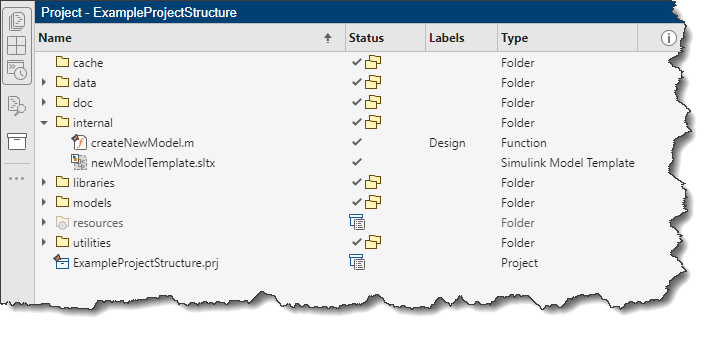
Today I am happy to welcome Sarah Dagen from MathWorks Consulting Services to talk about project organization.I recently received this email from a friend:I'm helping my friends get started with... read more >>
For a first post about R2025a, I decided to highlight 3 enhancements that will help speed up your Simulink workflows... and since it helped me writing this post, a quick mention of the new MATLAB... read more >>
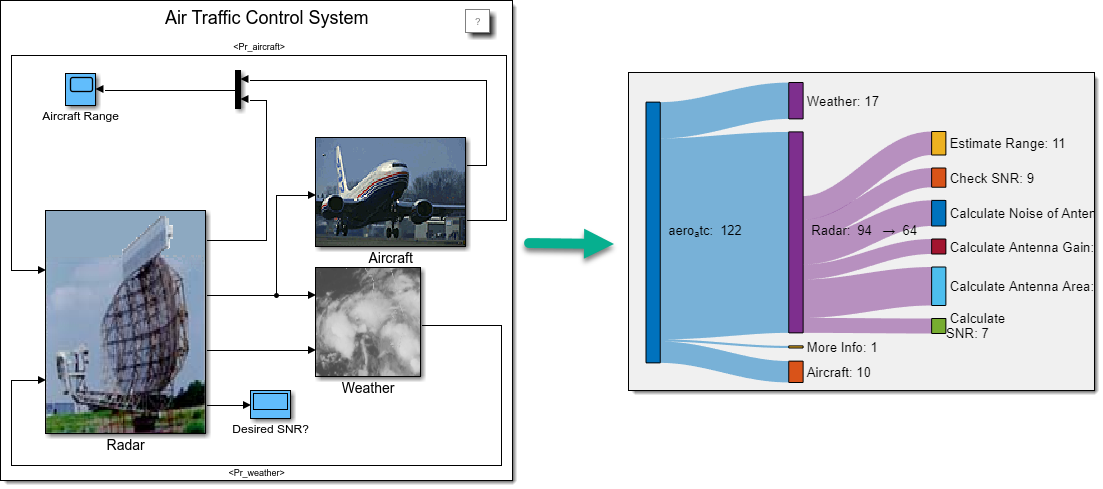
I was recently discussing different ways to visualize the content of a Simulink model with colleagues. Working in technical support, I receive models from users every day and it's always useful to... read more >>
These postings are the author's and don't necessarily represent the opinions of MathWorks.