About twelve years ago, I was implementing the algorithm that became roifill in the Image Processing Toolbox. In this algorithm, a specified set of pixels is replaced (or filled in) such that each of the replaced pixels equals the average of its north, east, south, and west neighbors. I had implemented an iterative algorithm, which worked but was slow. When I asked MATLAB creator and company cofounder Cleve if he knew a better way, he immediately replied, "It looks like a sparse linear system to me. Why don't you just use backslash?"

Head slap! Of course.

Now here I am again, looking at a very similar set of equations and thinking again about using sparse backslash.

In the Tarboton paper, the upslope area calculation is formulated recursively. That is, the upslope area of a pixel equals 1 plus some fraction of the upslope area of its neighboring pixels. (The specific fraction is a function of the flow direction for the neighbors.) So that's a linear system of equations. Let's see how to set up and solve the system in MATLAB.

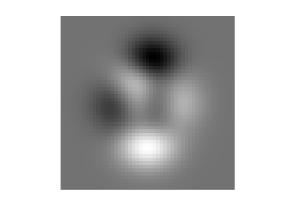
We'll start by making a test "DEM" to work with. I like using peaks.

E = peaks;
imshow(E, [], 'InitialMagnification', 'fit')

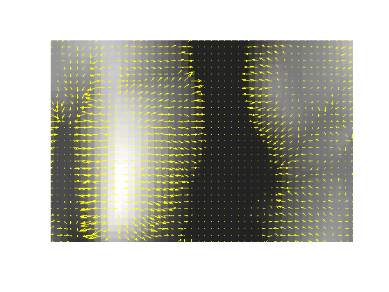
Next, compute the pixel flow directions, using the function dem_flow from my upslope area contribution on the MATLAB Central File Exchange.

R = dem_flow(peaks);

Each row and column of our sparse system will correspond to an individual pixel. It will be convenient to make a matrix, the same size as E, that "numbers" or labels the individual pixels of E. These labels will be used as the sparse matrix row and column coordinates.

pixel_labels = 1:numel(E);
pixel_labels = reshape(pixel_labels, size(E));
pixel_labels(1:4, 1:6)

ans =

     1    50    99   148   197   246
     2    51   100   149   198   247
     3    52   101   150   199   248
     4    53   102   151   200   249

Let's consider north neighbors. Here's the set of pixels with north neighbors:

pixels_with_north_neighbors = pixel_labels(2:end, :);

And here are the corresponding north neighbors:

north_neighbors = pixel_labels(1:end-1, :);

The angle pointing inward from a pixel's north neighbor to itself is -pi/2:

inward_angle = -pi/2;

A pixel's north neighbor has a flow that points in a particular direction. That direction is contained in R. If the flow direction is the same as the inward angle, then the fraction of flow from that neighbor is 1.0. If the flow direction is pointing more than pi/4 radians away from the inward angle, then the fraction of flow from that neighbor is 0.0. For inbetween angular differences, the fraction varies linearly from 1.0 to 0.0.

I have written simple functions to compute angular differences and the corresponding weights. The angular difference computation looks like this:

 d = mod(theta1 - theta2 + pi, 2*pi) - pi;

and the directional weight computation looks like this:

 w = max(1 - abs(d)*4/pi, 0);

With these functions, we can compute the north neighbor weights for all the pixels at once:

w = directional_weight(angular_difference(R(north_neighbors), ...
    inward_angle));

Ignoring the other neighbors for the moment, the upslope area equation looks like this:

  Ap = 1 + wAn

where Ap is the upslope area of the pixel, An is the upslope area of the north neighbor, and w is the directional weight based on the flow direction of the north neighbor. Rewrite the equation this way to see how to construct the linear equation matrix:

 Ap - wAn = 1

So each row of our matrix is going to have a 1 on the diagonal, and it's going to have the negative of the directional flow weights for each of its neighbors. If we used only the northern weights computed above, we could construct the sparse matrix this way:

i = pixels_with_north_neighbors(:);
j = north_neighbors(:);
w = w(:);

% Add diagonal terms
ii = [i ; pixel_labels(:)];
jj = [j ; pixel_labels(:)];
ww = [w ; ones(numel(pixel_labels), 1)];

% And construct the linear system matrix with a call to sparse
T = sparse(ii, jj, ww);
spy(T)

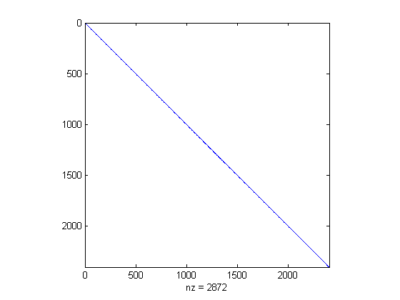
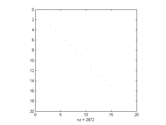
We have to zoom in to clearly see the off-diagonal terms:

xlim([0 20])
ylim([0 20])

I'm going to call T the flow matrix. To finish computing T, we'd have to repeat some of the steps above for each of the seven other neighbor directions, which is way too tedious to reproduce here. I'll just use the flow_matrix function in my MATLAB Central File Exchange submission:

T = flow_matrix(E, R);

Now we can compute the upslope area of each pixel by solving the matrix equation:

  Ta = b

where T is the sparse matrix we just formed, a is the vector of upslope areas for every pixel, and b is a vector of ones.

a = T \ ones(numel(E), 1);
A = reshape(a, size(E));

imshow(A, [], 'InitialMagnification', 'fit')

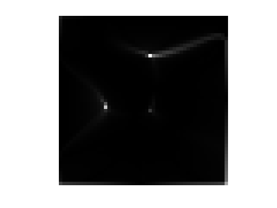
I have found that using log(A) works well for visualizing an upslope area matrix:

imshow(log(A), [], 'InitialMagnification', 'fit')

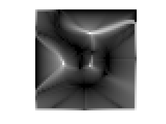
The brighter values have the highest upslope areas.

In my next post in this series, I'll revisit the issue of handling plateaus.

Get the MATLAB code

Published with MATLAB® 7.4