 Cleve’s Corner: Cleve Moler on Mathematics and Computing
 The MATLAB Blog
 Guy on Simulink
 MATLAB Community
 Artificial Intelligence
 Developer Zone
 Stuart’s MATLAB Videos
 Behind the Headlines
 File Exchange Pick of the Week
 Hans on IoT
 Student Lounge
 MATLAB ユーザーコミュニティー
 Startups, Accelerators, & Entrepreneurs
 Autonomous Systems
 Quantitative Finance
 MATLAB Graphics and App Building
Relationship between continuous-time and discrete-time Fourier transforms
Previously in my Fourier transforms series I've talked about the continuous-time Fourier transform and the discrete-time Fourier transform. Today it's time to start talking about the relationship between these two.
Let's start with the idea of sampling a continuous-time signal, as shown in this graph:

Mathematically, the relationship between the discrete-time signal and the continuous-time signal is given by:

(When I write equations involving both continuous-time and discrete-time quantities, I will sometimes use a subscript "c" to distinguish them.)
The sampling frequency is  (in Hz) or
  (in radians per second).
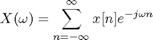
The discrete-time Fourier transform of  is related to the continuous-time Fourier transform of
  as follows:
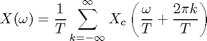
But what does that mean? There are two key pieces to this equation. The first is a scaling relationship between  and
and  :
:  . This means that the sampling frequency in the continuous-time Fourier transform,
  , becomes the frequency
  in the discrete-time Fourier transform. The discrete-time frequency
  corresponds to half the sampling frequency, or
  .
.
The second key piece of the equation is that there are an infinite number of copies of  spaced by .
Let's look at a graphical example. Suppose  looks like this:
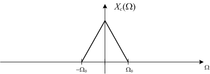
Note that equals zero for all frequencies  . This is what we mean when we say a continuous-time signal is band-limited. The frequency
  is called the bandwidth of the signal.
The discrete-time Fourier transform of looks like this:
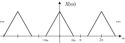
where  . As I mentioned before, normally only one period of
  is shown:
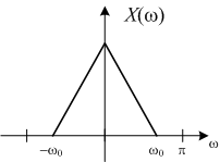
For this example, then, between  and
and  looks just like a scaled version of .
Next time we'll consider what happens when doesn't look like . In other words, we're about to tackle aliasing.
- Category:
- Fourier transforms


Comments
To leave a comment, please click here to sign in to your MathWorks Account or create a new one.