Steve on Image Processing

I'd like to welcome back guest blogger Brett Shoelson for the continuation of his series of posts on implementing image special effects in MATLAB. Brett, a contributor for the File Exchange Pick of the Week blog, has been doing image processing with MATLAB for almost 20 years now.

[Part 1] [Part 2] [Part 3] [Part 4]

Contents

Put Me In the Zoo!

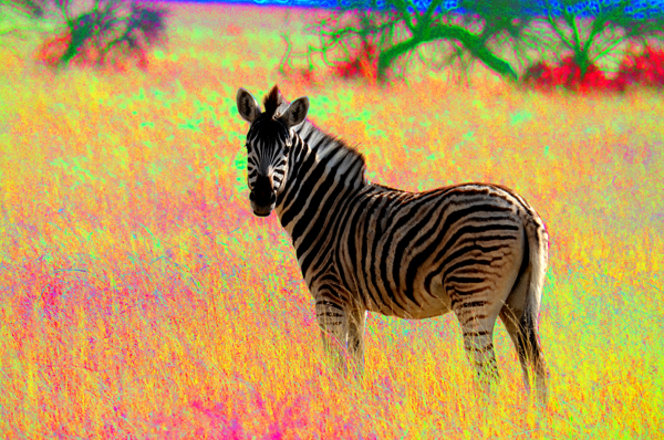
So far (post 1, post 2) in this guest series on creating special image effects with MATLAB, I've applied processes to the entire image. For instance, I created the image above by starting with the contrast-enhanced elephant from my previous post. I created the pseudocolor effect by decorrelation-stretching (using decorrstretch) the resulting image. And then I enhanced the colors a bit using imadjust.

URL = 'http://blogs.mathworks.com/pick/files/ElephantProfile.jpg';
img = imread(URL);
colorElephant = decorrstretch(img);
colorElephant = imadjust(colorElephant,[0.10; 0.79],[0.00; 1.00], 1.10);

(Decorrelation stretching is useful for visualizing, and sometimes analyzing, imagery by reducing inter-plane autocorrelation levels in an image. It is often used with multispectral or hyperspectral images.)

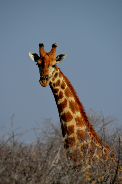
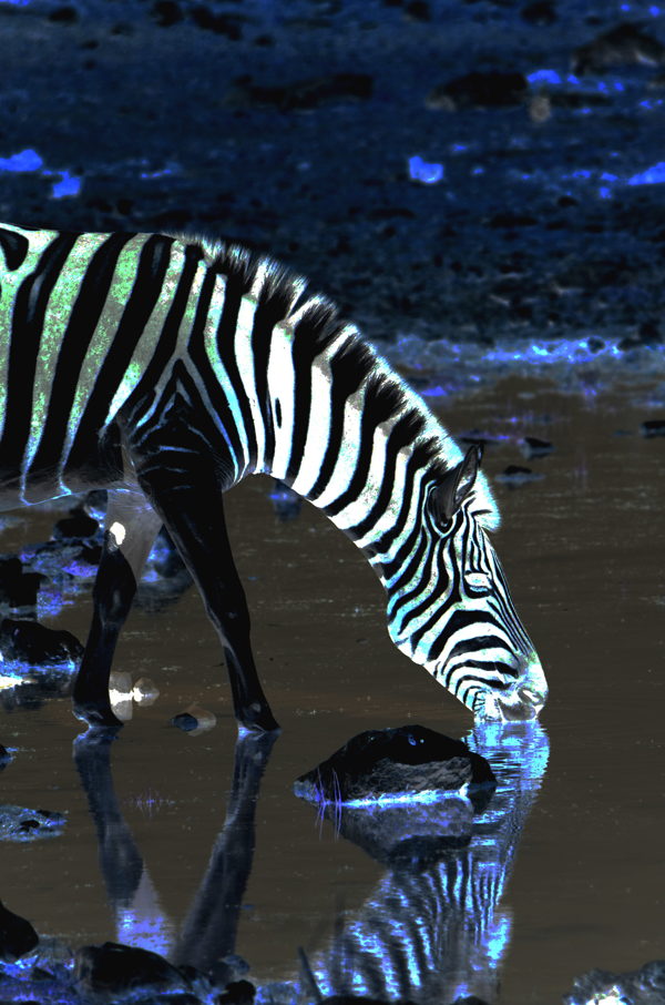
In this installment, I wanted to take an ordinary photograph of a giraffe and modify it to give the giraffe something out-of-the-ordinary. But to do so, I needed to segment the image--to create a binary mask with 1's in the locations of my regions of interest, and 0's elsewhere. There are many approaches to segmenting images--indeed, there are many approaches in the Image Processing Toolbox. So if we wanted to color the spots of a giraffe, for instance, we'd first have to find an appropriate method of segmenting the spots. (Without a doubt, getting a good segmentation is the most difficult part of many image processing problems!)

First, let's read and adjust the image of the giraffe.

URL = 'http://blogs.mathworks.com/pick/files/GiraffeProfile.jpg';
img = im2double(imread(URL));
img = imadjust(img,[0.20; 0.80],[0.00; 0.80], 1.10);
hAx = axes; %Notice that I created a handle to the axes; I will use that later.
imshow(img);

Next, I want to segment the giraffe's spots. Usually (but not always), when I'm trying to segment an RGB image, I find I can get a good mask working with one (or sometimes multiple) grayscale representation(s) of the color images. I like to look at the individual colorplanes and at different colorspace representations of the image as well. ExploreRGB makes that exploration easy:

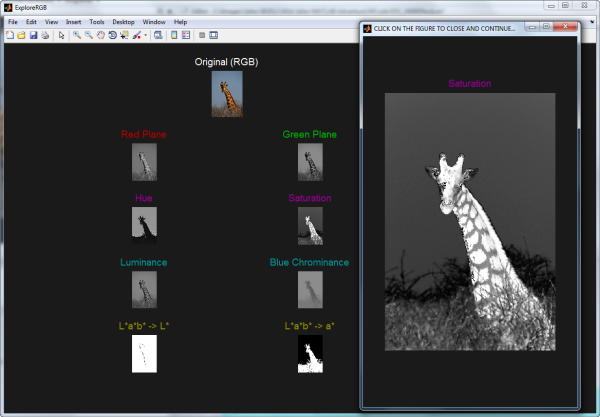
As we can see in this image of the ExploreRGB GUI, the giraffe's spots are fairly well segmented for us in the "saturation" plane of the HSV colorspace. So let's start there for our segmentation of the spots.

grayImg = rgb2hsv(img);
grayImg = grayImg(:,:,2);
grayImg =  imadjust(grayImg,[0.6; 1.0],[0.00; 1.00], 1.00);
spotMask = im2bw(grayImg,graythresh(grayImg));

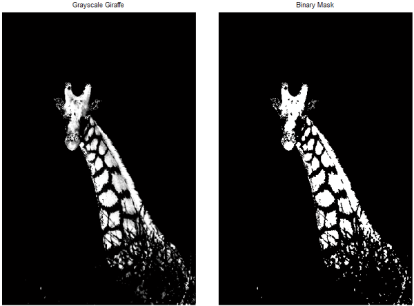
Now, if I were happy with that as a segmentation mask, I could move on. But I only wanted the giraffe's spots--not its head or mane. I could continue to try different programmatic approaches; remember that I can combine these logical masks in any way that makes sense. But instead, I'm going to take my first cue from Photoshop and go old-school: I'm going to manually exclude the portions of the giraffe that I don't want to colorize. So how do I do that?

imfreehand to the Rescue!

A few years back (R2008a, I believe), we refactored our region-of-interest (ROI) tools. I want to draw a freehand region, and use it to help mask my image. So, using imfreehand, I quickly encircle the region I want to exclude. (I say "quickly," but you generally want to take your time with this step; getting a good segmentation mask is crucial to getting a good effect!)

To create the manual mask:

manualMask = imfreehand;
posns = getPosition(manualMask);
[m,n,~] = size(grayImg);
excludeMask = poly2mask(posns(:,1),posns(:,2),m,n);

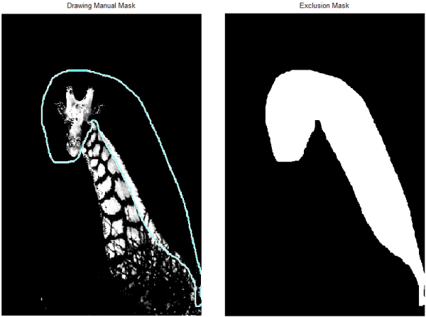
Now I can combine that with my original spot mask, with the logical combination "...AND NOT....":

spotMask  = spotMask & ~excludeMask;

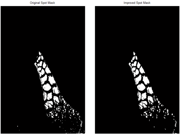
In displaying the result (below left), I recognize that I trimmed the mask manually a bit tighter than I intended, so I will dilate it a bit (imdilate), and then exclude small regions (fewer than 10 connected pixels) using bwareaopen. The result is shown below on the right.

spotMask  = spotMask & imdilate(~excludeMask,strel('disk',2));
spotMask = bwareaopen(spotMask,10);

That's close to my desired mask, but I'm going to tweak it a bit more by filling holes in the spots (imfill) and by manipulating it with some morphological operations (MorphTool again!). One more application of bwareaopen (this time, keeping only very large blobs), and I have the segmentation mask looking the way I want it.

spotMask = imfill(spotMask,'holes');
spotMask = imopen(spotMask,strel('disk',10));
spotMask = imdilate(spotMask,strel('disk',10));
spotMask = bwareaopen(spotMask,2000);

Now to Color the Spots

From this point, coloring the spots was reasonably straightforward: I simply labeled the spots (bwlabel) and colored the labeled regions by calling label2rgb. (Also, I specified "jet" as my colormap and used the "shuffle" command to randomly assign map colors to the spots.) Next, I set the "hold" property of the current axes (i.e., the one containing the original color image), and displayed the colored spots on top of the original image. Finally, I modified the "alphadata" property of the colored-spot image to set its transparency to 0.25.

L = bwlabel(spotMask);
colormask = label2rgb(L,jet(max(L(:))),[0 0 0],'shuffle');
% Using the handle to the axes that contains the original image, make
% that axes current, and set its "hold" property on.
axes(hAx)
hold on
h = imshow(colormask); %I created a handle here, too.
colortrans = 0.25;
set(h,'alphadata',colortrans);

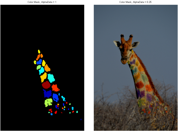
Now all that remains is to capture the visualization as an RGB image. I'm simply going to start with a copy of the original giraffe image, and modify it colorplane-by-colorplane, scaling each by 0.75 (i.e., 1-colortrans) and adding the scaled RGB components of the colored-spot image:

imgEnhanced = img;
for ii = 1:3
   imgEnhanced(:,:,ii) = img(:,:,ii)*(1-colortrans) + im2double(colormask(:,:,ii))*colortrans;
end

Next Up: Out Standing in the Field

All images copyright Brett Shoelson; used with permission.

Get the MATLAB code

Published with MATLAB® R2012b

Published with MATLAB® R2012b