
The time has come! After more than 30 years of software development at MathWorks, I have decided to retire. Friday, March 29, will be my last day. For 18 of those 30 years, I’ve been writing... read more >>

Note
Steve on Image Processing with MATLAB has been archived and will not be updated.
The time has come! After more than 30 years of software development at MathWorks, I have decided to retire. Friday, March 29, will be my last day. For 18 of those 30 years, I’ve been writing... read more >>


While I was working on a prototype yesterday, I found myself writing a small bit of code that turned out to be so useful, I wondered why I had never done it before. I'd like to show it to you.... read more >>

Today's post is by guest blogger Isaac Bruss. Isaac has been a course developer for MathWorks since 2019. His PhD is in computational physics from UMass Amherst. Isaac has helped launch and support... read more >>

For some shapes, especially ones with a small number of pixels, a commonly-used method for computing circularity often results in a value which is biased high, and which can be greater than 1. In... read more >>
I have seen some requests and questions related to identifying objects in a binary image that are touching the image border. Sometimes the question relates to the use of imclearborder, and... read more >>
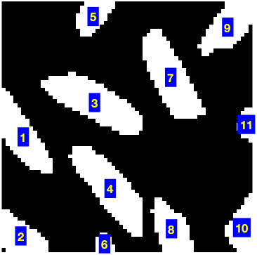
Someone recently asked me about the order of objects found by the functions bwlabel, bwconncomp, and regionprops. In this binary image, for example, what accounts for the object order?The functions... read more >>

In May 2006, I wrote about a technique for computing fast local sums of an image. Today, I want to update that post with additional information about integral image and integral box filtering... read more >>

In some of my recent perusal of image processing questions on MATLAB Answers, I have come across several questions involving binary image objects and polygonal boundaries, like this.The questions... read more >>
Note added 20-Dec-2022: I wrote this post with lossy JPEG in mind. If you work with DICOM data, see Jeff Mather's note in the comments below about the use of lossless JPEG in DICOM. I have... read more >>
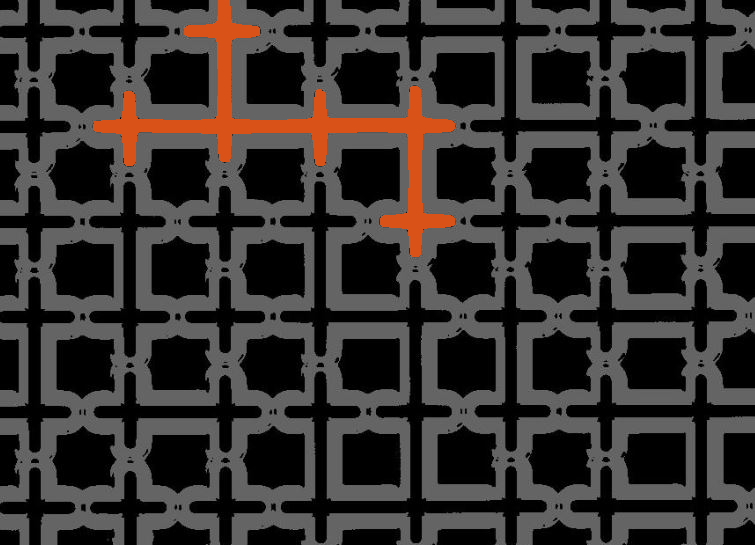
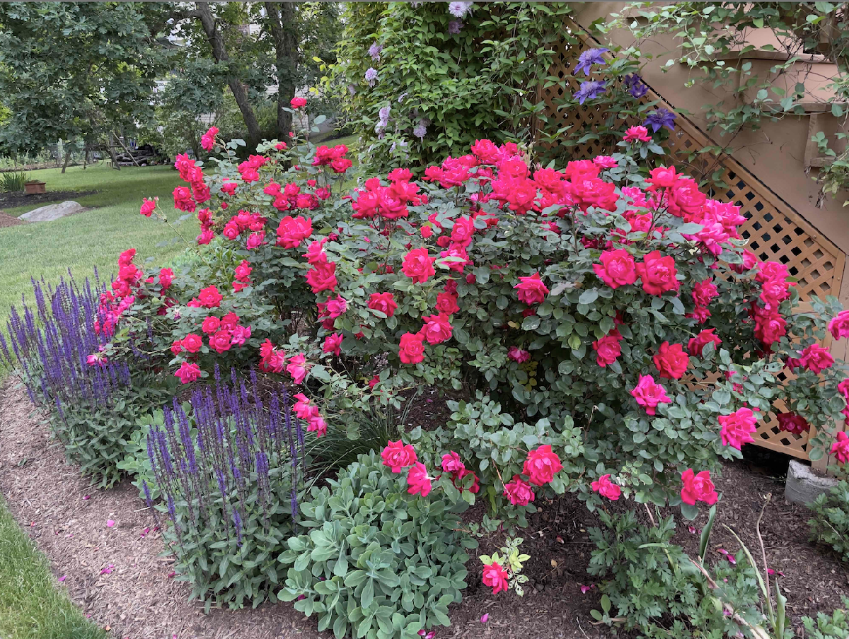
Last winter, Aktham asked on MATLAB Answers how to find the channels in this image.url = "https://www.mathworks.com/matlabcentral/answers/uploaded_files/880740/image.jpeg";A =... read more >>
These postings are the author's and don't necessarily represent the opinions of MathWorks.