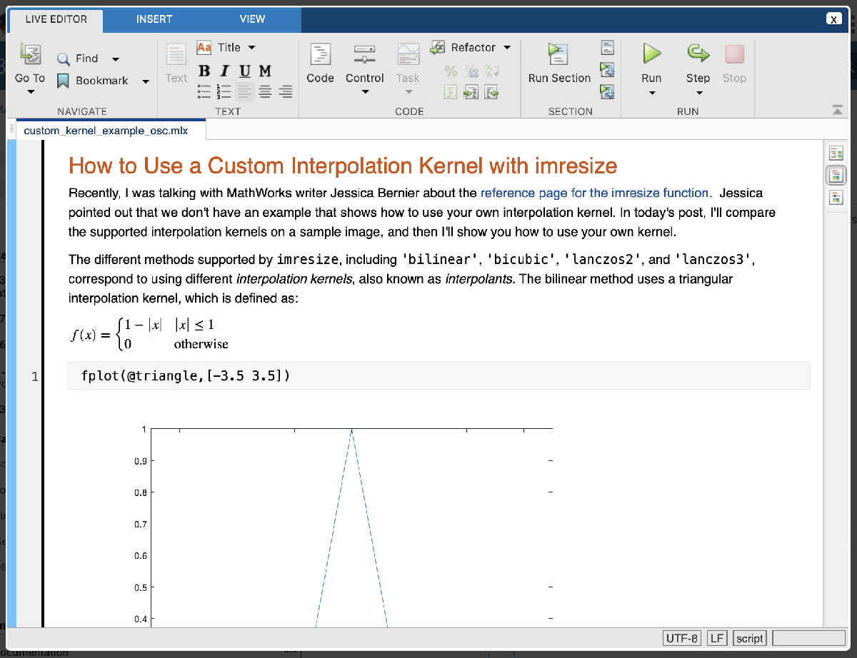
Recently, I was talking with MathWorks writer Jessica Bernier about the reference page for the imresize function. Jessica pointed out that we don't have an example that shows how to use your own... read more >>

I have published more than 560 blog posts here since 2006, and I estimate that about 98% of them started out as MATLAB scripts.Recently, I've started writing my blog posts as live scripts. Live... read more >>

Today's blog post comes from planning one topic, but then taking a sharp left turn and doing something else completely. I was thinking about writing something related to meshgrid, and so I was... read more >>

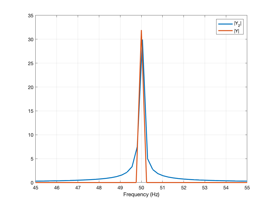
A MATLAB user recently contacted MathWorks tech support to ask why the output of fft did not meet their expectations, and tech support asked the MATLAB Math Team for assistance. Fellow Georgia Tech... read more >>

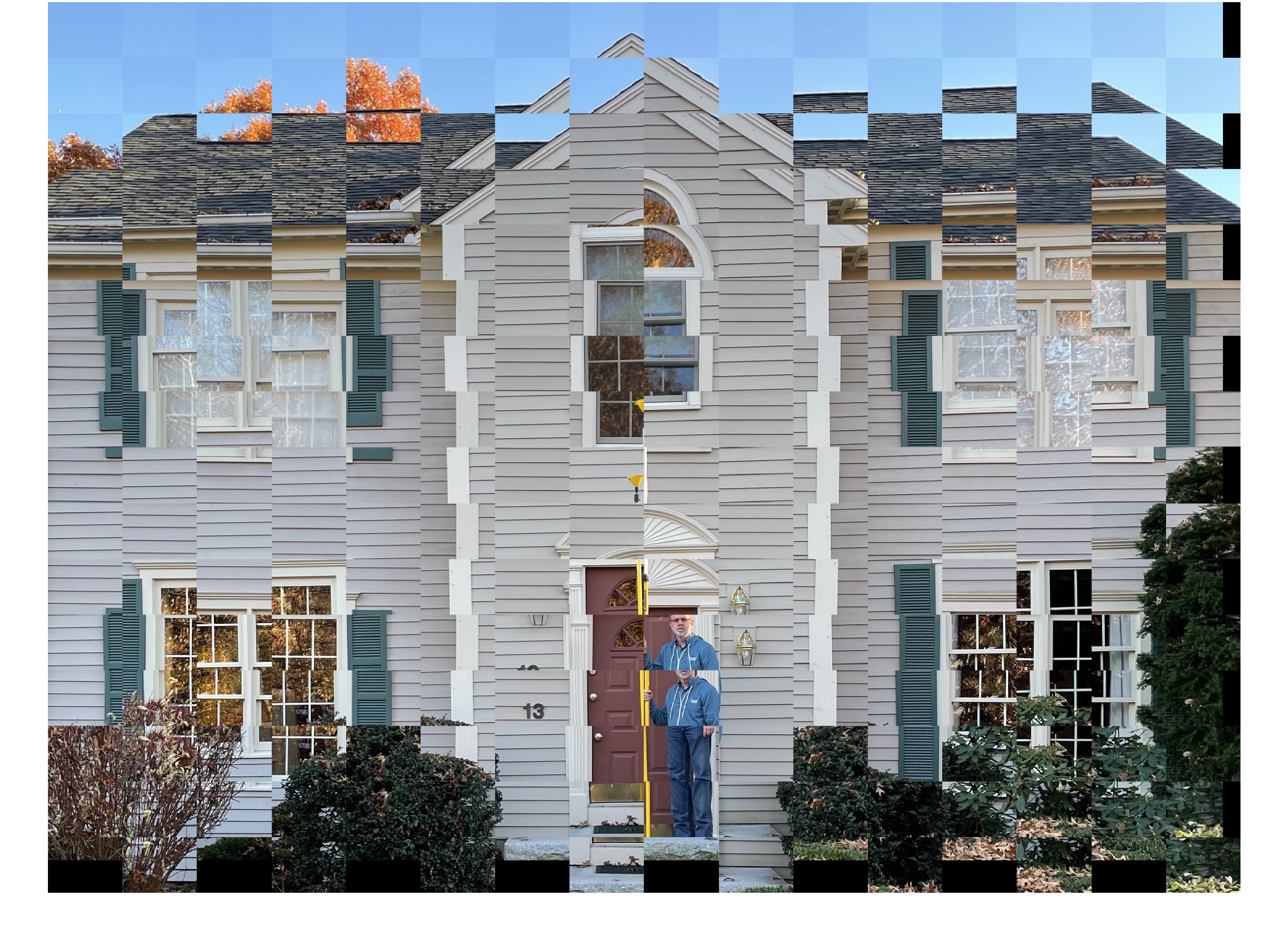
In this post, I'll explore how imshowpair and imfuse work.Reason: I was curious.Last month, I wrote about registering several hand-held photographs together. In that post, I used imshowpair several... read more >>

The typical modern French* horn, pictured below, has about 23 total feet of tubing. At the beginning and the end, the tubing is conical. In the middle, the tubing is cylindrical.Depending on which... read more >>

A question on MATLAB Answers caught my eye earlier today. Borys has this pseudocolor image of a weighted adjacency matrix: And he has this image of the color scale: Borys wants to know how to compute... read more >>

I wrote previously about the new colorChecker, which can detect X-Rite test charts in the R2020b release. Another area of new color-related functionality is computing perceptual color differences.... read more >>

Lately, I've been spending more time on MATLAB Central, and I'd like to encourage you to try out some of the resources there, if you haven't already.Have you heard of Cody? It is an addictive MATLAB... read more >>

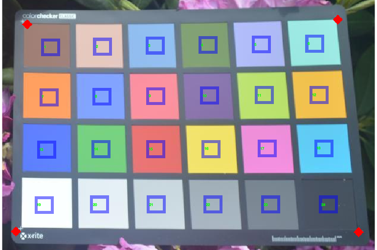
When I saw this picture, I was really tempted to take it into the local garden nursery and ask them how to keep color checker charts out of my rhododendrons. No, no, this post is not really about... read more >>