 Cleve’s Corner: Cleve Moler on Mathematics and Computing
 The MATLAB Blog
 Guy on Simulink
 MATLAB Community
 Artificial Intelligence
 Developer Zone
 Stuart’s MATLAB Videos
 Behind the Headlines
 File Exchange Pick of the Week
 Hans on IoT
 Student Lounge
 MATLAB ユーザーコミュニティー
 Startups, Accelerators, & Entrepreneurs
 Autonomous Systems
 Quantitative Finance
 MATLAB Graphics and App Building
Dark Energy Gravitational Waves
Recent theoretical, observational and computational results establish the possibility that gravitational waves produced by the dark energy created at the dawn of the universe affect the clock rate of silicon digital processors operating at very low temperatures.
Contents
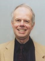
Ed Plum
Ed Plum is a professor in the Institute for Theoretical Physics at the U. C. Santa Barbara. He is also a long-time friend of mine and an avid MATLAB fan.
Ed and his colleagues are publishing an important paper today. Here is a link to the journal, Physical Review Communications. Ed has shared an advanced copy with me. They have found convincing evidence that the gravitational waves predicted by Einstein's General Theory of Relativity and emanating from "Dark Energy" affect the operating frequency of silicon computer chips. The effect can be observed in experiments operating at temperatures below 2 degrees Kelvin.
LIGO
The announcement on February 11 of the detection of gravitational waves by the LIGO team thrilled scientists and the public at large worldwide. LIGO stands for Laser Interferometer Gravitational-Wave Observatory. Here is the link to the LIGO home page. Here is their scientific paper in Physical Review Letters. Excellent survey articles were published in The New York Times Sunday Review and The New Yorker.
Here is a Wikipedia animated graphic depicting gravitational waves in the article on General Relativity.
LIGO Labs
The LIGO experiment is designed to detect powerful one-time astrophysical events such as colliding black holes. The gravitational waves involved have wave lengths that require L-shaped detectors with legs four kilometers long. A wave passes through the detector just once, in a fraction of a second. There are two detectors, located in Washington State and Louisiana.

Photo: <http://www.ligo.caltech.edu >
LIGO Gravitational Waves
This beautiful graphic from the Phys. Rev. Letters paper shows the event detected by the LIGO team. The top two figures show the actual signals recorded at the two labs. The next two figures show the results from supercomputer runs for the numerical solution of Einstein's equations. The small pair of figures show that the difference between the observations and the simulations is noise. The two color figures show the "chirps", spectrograms plotting frequency versus time. These chirps are readily audible to the human ear.

Source: <http://www.ligo.caltech.edu>
Dark Energy Gravitational Waves
The most commonly accepted model of cosmology hypothesizes dark energy, formed at the origin of the universe and permeating all of space, but invisible to optical observation. According to Einstein's General Theory of Relativity, this energy constantly produces short wave length, very low energy gravitational waves. These waves continuously interact with all mass in the universe, but on a scale that is almost impossible to detect.
Plum and his colleagues have evidence from both numerical simulations and actual observations that the dark energy gravitational waves affect the operating frequency of commercial microprocessors. Very slight changes in processor speed can be detected, provided the silicon is exceptionally pure and the observations are made at very low temperatures. It's like immersing a high-end laptop in liquid nitrogen. Here is one of the detectors.

Photo: Plum et al
The signal
Some time ago, Ed gave me access to one of the first signals his group had detected and we have been quietly including it as one of sample sounds on recent MATLAB distributions. The file is chirp.mat. We have reversed the signal to disguise it until now. You should be able to load a copy on your own machine.
    clear
    which chirp.mat
    load chirp.mat
    y = flipud(y)';
    t = (1:length(y))/Fs;
    whos
C:\Program Files\MATLAB\R2016a\toolbox\matlab\audiovideo\chirp.mat
  Name      Size                Bytes  Class     Attributes

  Fs        1x1                     8  double
  t         1x13129            105032  double
  y         1x13129            105032  double
The first plot is the entire signal. Since the waves are arriving continuously, we see several peaks. The second plot zooms in on one of the peaks.
    subplot(2,1,1)
    plot(t,y)
    axis([0 t(end) -1 1])

    subplot(2,1,2)
    plot(t,y)
    axis([.75 .80 -1 1])
    xlabel('Time (secs)')

The sound
I hope you can run this sound yourself and hear the chirps. If you are just reading this on the Web, you will have to imagine what this sounds like.
sound(y,Fs)
The spectrogram
Here is the picture of one chirp, the spectrogram of about one-eighth of the signal.
    clf reset
    spectrogram(y(1:2048),kaiser(128,18),120,128,Fs,'yaxis')

Expectations
This is just be beginning. We expect to learn much more about our universe as we are able to refine the silicon in the microprocessors and lower the temperature of the operating environment.


Comments
To leave a comment, please click here to sign in to your MathWorks Account or create a new one.