Upslope area – Plateau processing
[NOTE: After I originally wrote this post about handling plateaus, I discovered problems with the method, so I am no longer using it. I revisited the plateau issue in a later post. -SE]
Today I'll continue thinking about plateaus in a DEM and what they mean for calculating pixel flow. Here's a very tiny portion of my DEM array, just northwest of North Pond.
a = [120 118 123; 120 118 125; 119 119 126]
a =

   120   118   123
   120   118   125
   119   119   126
The center pixel doesn't have a downhill neighbor, so I'm calling it a plateau pixel. No matter that it's a very small plateau; we can't compute a pixel flow direction for it, and that will cause problems when we get around to computing upslope area.
One technique used in image processing to deal with plateaus is called the lower complete transformation. A lower complete image is one where the only pixels having no downhill neighors are the pixels belonging to regional minima. Roughly speaking, the lower complete transformation operates by elevating plateau pixels. Pixels further from the plateau edge get elevated more. Of course, pixels uphill from the plateau need to be elevated as well so that they remain uphill. I have read about this technique but have never implemented it myself. (For more information, I recommend P. Soille, Morphological Image Analysis: Principles and Applications, 2nd edition, Springer, 2003, pp. 222-226.)
I'm going to use a different technique, one that's based on the algorithm in the Image Processing Toolbox function roifill. This function fills in pixels in a particular region by smoothly interpolating from the pixels surrounding the region. It does so by solving a sparse linear system based on the notion that, in the filled output, each pixel in the filled region equals the average of its north, east, south, and west neighbors. (It's kind of an interesting method. Maybe that'll be a future blog topic.)
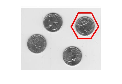
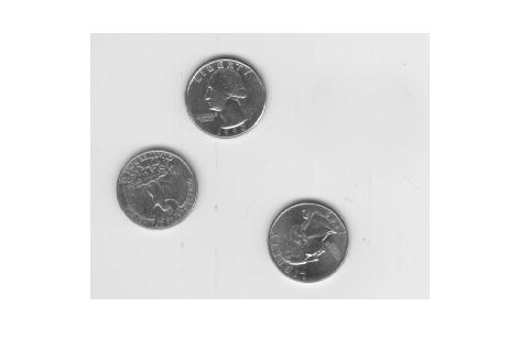
Here's the example (slightly modified) from the roifill documentation:
I = imread('eight.tif');
imshow(I)

c = [222 272 300 270 221 194 222];
r = [21 21 75 121 121 75 21];
hold on
plot(c,r,'r','LineWidth',4)

J = roifill(I,c,r);
imshow(J)

And here's what roifill does to our tiny snippet from the DEM:
mask = true(3, 3);
b = roifill(a, mask)
b =

  120.0000  118.0000  123.0000
  120.0000  120.5000  125.0000
  119.0000  119.0000  126.0000
You can see that the center pixel has been replaced by a new value, and that the center pixel now has a downhill neighbor.
Here's a slightly bigger example, where the two center pixels have no downhill neighbors:
a2 = pond(15:17, 19:22)
a2 =

   116   116   116   120
   117   115   115   117
   119   115   115   116
And the output of roifill
mask2 = true(3, 4);
b2 = roifill(a2, mask2)
b2 =

   116   116   116   120
   117   116   116   117
   119   115   115   116
Well, the two center pixels now have downhill neighbors, but WAIT! The (1,2) pixel no longer has a downhill neighbor! OK, time to 'fess up. I didn't really anticipate that this would be a problem. I'll have to give this some thought. My first reaction is: It'll be OK because we can use the original, unmodified DEM values to compute the pixel flow for the nonplateau pixels. We only need the modified DEM values to compute pixel flow for the plateau pixels. But I'll sleep on it.
Assuming I can resolve that problem successfully, we can use roifill to compute pixel flow directions for the midplateau pixels. It won't help us, though, for the plateau pixels that are part of regional maxima or regional minima. I'll figure out what to do about those next week.
- 类别:
- Upslope area
 Cleve’s Corner: Cleve Moler on Mathematics and Computing
 The MATLAB Blog
 Guy on Simulink
 MATLAB Community
 Artificial Intelligence
 Developer Zone
 Stuart’s MATLAB Videos
 Behind the Headlines
 File Exchange Pick of the Week
 Hans on IoT
 Student Lounge
 MATLAB ユーザーコミュニティー
 Startups, Accelerators, & Entrepreneurs
 Autonomous Systems
 Quantitative Finance
 MATLAB Graphics and App Building


评论
要发表评论,请点击 此处 登录到您的 MathWorks 帐户或创建一个新帐户。