Filtering fun
Today I want to take the test pattern I created last time and subject it to a variety of frequency-based filters.
In this post I'll be using a variety of frequency design and frequency-response visualization tools in MATLAB, Signal Processing Toolbox, and Image Processing Toolbox, including fir1, ftrans2, freqspace, fwind1, and freqz2. I won't be giving much explanation of these filter design techniques. Perhaps in the future I'll explore filter design here in more detail. For now, though, I really just want to have some fun with this test pattern.
[x,y] = meshgrid(-200:200);
r = hypot(x,y);
km = 0.8*pi;
rm = 200;
w = rm/10;
term1 = sin( (km * r.^2) / (2 * rm) );
term2 = 0.5*tanh((rm - r)/w) + 0.5;
g = (term1 .* term2 + 1) / 2;

imshow(g, 'XData', [-.8 .8], 'YData', [-.8 .8])
axis on
xlabel('Normalized frequency'), ylabel('Normalized frequency')
title('Test pattern')
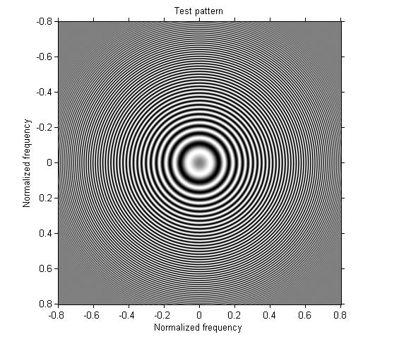
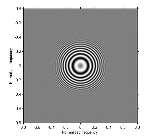
Example 1: Design a one-dimensional lowpass filter and apply it in both directions.
b = fir1(30,0.3);
h = b' * b;
g1 = imfilter(g, h);

imshow(g1, 'XData', [-.8 .8], 'YData', [-.8 .8])
axis on
xlabel('Normalized frequency'), ylabel('Normalized frequency')
Example 2: Design a one-dimensional highpass filter and apply it in both directions.
b2 = fir1(30, 0.3, 'high');
h2 = b2' * b2;
g2 = imfilter(g, h2);

imshow(g2, [], 'XData', [-.8 .8], 'YData', [-.8 .8])
axis on
xlabel('Normalized frequency'), ylabel('Normalized frequency')
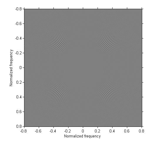
Example 3: Design a one-dimensional bandpass filter and apply it on both directions.
b3 = fir1(30, [0.3 0.4]);
h3 = b3' * b3;
g3 = imfilter(g, h3);

imshow(g3, [], 'XData', [-.8 .8], 'YData', [-.8 .8])
axis on
xlabel('Normalized frequency'), ylabel('Normalized frequency')

Example 4: Apply the one-dimensional bandpass filter from the previous step in only one direction.
g4 = imfilter(g, b3);

imshow(g4, [], 'XData', [-.8 .8], 'YData', [-.8 .8])
axis on
xlabel('Normalized frequency'), ylabel('Normalized frequency')

Example 5: Use ftrans2 to turn the one-dimensional bandpass filter from the previous example into a two-dimensional bandpass filter that is approximately circularly symmetric.
h5 = ftrans2(b3);
g5 = imfilter(g, h5);

imshow(g5, [], 'XData', [-.8 .8], 'YData', [-.8 .8])
axis on
xlabel('Normalized frequency'), ylabel('Normalized frequency')

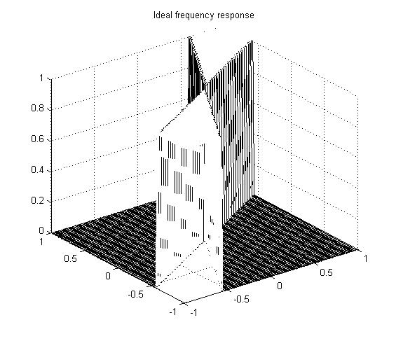
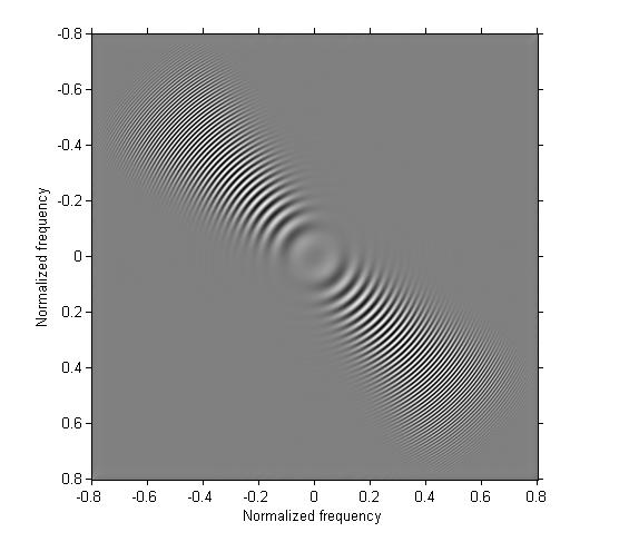
Example 6: Use fwind1 to design a two-dimensional filter that has a wedge-shaped frequency response.
[f1, f2] = freqspace(101, 'meshgrid');
theta = cart2pol(f1, f2);
Hd = ((theta >= pi/6) & (theta < pi/3)) | ...
    ((theta >= -5*pi/6) & (theta < -2*pi/3));
mesh(f1, f2, double(Hd))
title('Ideal frequency response')
h6 = fwind1(Hd, hamming(31));
freqz2(h6)
title('Designed filter frequency response')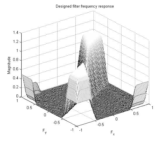
g6 = imfilter(g, h6);

imshow(g6, [], 'XData', [-.8 .8], 'YData', [-.8 .8])
axis on
xlabel('Normalized frequency'), ylabel('Normalized frequency')
Example 7: Compare the use of an averaging filter and a Gaussian filter. This example is inspired by Cris Luengo's comment from last week.
g7 = imfilter(g, fspecial('average', 9));
imshow(g7, [], 'XData', [-.8 .8], 'YData', [-.8 .8])
axis on
xlabel('Normalized frequency'), ylabel('Normalized frequency')
title('13-by-13 averaging filter')
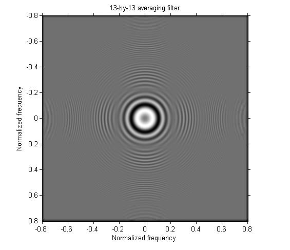
You can see that some very high frequencies remain in the output. The Gaussian filter performs much better:
g9 = imfilter(g, fspecial('gaussian', 9, 2));
imshow(g9, [], 'XData', [-.8 .8], 'YData', [-.8 .8])
axis on
xlabel('Normalized frequency'), ylabel('Normalized frequency')
title('13-by-13 Gaussian filter')

OK, I'm going to give this test pattern a rest for now. Phew!
 Cleve’s Corner: Cleve Moler on Mathematics and Computing
 The MATLAB Blog
 Guy on Simulink
 MATLAB Community
 Artificial Intelligence
 Developer Zone
 Stuart’s MATLAB Videos
 Behind the Headlines
 File Exchange Pick of the Week
 Hans on IoT
 Student Lounge
 MATLAB ユーザーコミュニティー
 Startups, Accelerators, & Entrepreneurs
 Autonomous Systems
 Quantitative Finance
 MATLAB Graphics and App Building




コメント
コメントを残すには、ここ をクリックして MathWorks アカウントにサインインするか新しい MathWorks アカウントを作成します。