Dealing with “Really Big” Images: Block Processing
I'd like to welcome back guest blogger Brendan Hannigan, for the second in a series of three posts on working with very large images in MATLAB.
Contents
- Dealing with "Really Big" Images: Block Processing
- "Sounds good. let's do this!"
- "This seems familiar to me..."
- "Wait, didn't I read on CSSM that blockproc is way slower than blkproc ?"
- "What just happened?"
- "Uhm... 'block struct'? That seems overly complicated"
- "What's with those lines all over your result?"
- "Ok, so how do I fix it?"
- "Ok great, you fixed it. What does this have to do with large images?"
- "Hmm, ok yea that's cool. What's the catch?"
- "You're killing me with these file format restrictions! I don't use TIFF!"
Dealing with "Really Big" Images: Block Processing
Hi! This is Brendan Hannigan, back again to continue our discussion on working with very large images in MATLAB. In the previous blog I discussed a couple of different ways to view and explore large images using the Image Processing Toolbox. Today I'll take the next logical step down the "large image workflow" path and we'll explore how to process images that are too large to load into memory.
"Sounds good. let's do this!"
Since the entire image cannot be loaded into memory at one time, we opted for an incremental, file-to-file solution. Basically we want to read a part of your "input" image into memory, process it in some way, and then write the results back to a new file, the "output" image. We continue to do this until the entire image has been processed, avoiding Out of Memory errors.
"This seems familiar to me..."
The flow of data described here is very similar to an existing IPT function, blkproc, which allows for block processing of images, but like most other IPT functions, it only supports in-memory processing. Originally, we considered expanding the scope of blkproc to support file-to-file workflows as well, but there were some syntactic and behavioral issues that I wasn't comfortable with and we would've likely introduced some backwards incompatibilities.
We instead opted for a completely new function in release R2009b. The result? blockproc! Very creative name right? blockproc has all of the capabilities of blkproc and a LOT more!
"Wait, didn't I read on CSSM that blockproc is way slower than blkproc ?"
Ahem... well... Ok fine, yes, it USED to be slower. The initial release of blockproc went out with what I will refer to simply as "performance growth opportunities" (sorry about that).
However, with the release of R2010b, all that has changed! blockproc performance was dramatically improved and is now comparable with blkproc for similar tasks.
Let's have a quick look at how it works!
% read input image
A = imread('peppers.png');
imshow(A);
% define block size and function to run on each block of data
block_size = [64 64];
my_function = @(block_struct) block_struct.data(:,:,[3 2 1]);
% call blockproc!
B = blockproc(A,block_size,my_function);
figure;
imshow(B);
"What just happened?"
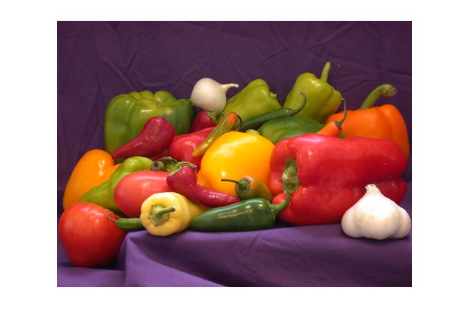
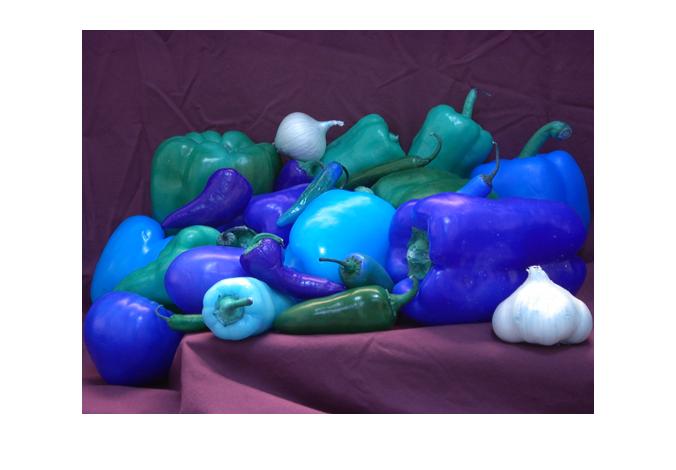
What we've done here is swapped the red and blue color channels of our RGB peppers image with some simple indexing. blockproc did this one 64x64 block at a time and assembled the results into a single output image. Things that were "mostly red" became "mostly blue" and vice versa while the purple background remained mostly unchanged.
Basically all blockproc needs is an input image, a block size, and a function handle to run (similar to blkproc);
You may notice that I used an "anonymous function" to create the function handle my_function, but that's not necessary. You can also provide a function handle to a function that's either defined on your path or sitting in your current directory. The only requirement is that the function must accept a "block struct" as it's sole input argument (that we will pass to it, from inside of blockproc), and must return the processed data.
"Uhm... 'block struct'? That seems overly complicated"
The block struct is a MATLAB struct that contains the block's image data (in the .data field) as well as several other pieces of useful information. Most important among these is the .location field, which contains the location (in your input image) where the block came from. This .location information opens up a vast new world of potential uses for blockproc that we won't get into here.
Most of the time you use blockproc you'll probably just use the .data field, but for any operation that changes depending on which block of the image you are processing, the .location field is key, and you'll be thanking me then! You can check out the blockproc doc to learn more about what other information we package into the block struct.
Now for a more "real" example, applying a low-pass filter to an image. First, the conventional way:
% read the original photo into memory
origp = imread('cameraman.tif');
imshow(origp);
% create a Gaussian low-pass filter
h = fspecial('gaussian',5,2);
% compute the derived photo
derp1 = imfilter(origp,h);
imshow(derp1);

Now, with blockproc. We will re-use the original photo, origp, as well as the Gaussian filter.
% create a function handle that we will apply to each block
myFun = @(block_struct) imfilter(block_struct.data,h);
% setup block size
block_size = [64 64];
% compute the new derived photo
derp2 = blockproc(origp,block_size,myFun);
imshow(derp2);

"What's with those lines all over your result?"
What we see here are artifacts from block processing. What happened? Well, as our function, imfilter, processes its input it will require some padding values near the edges of the image. By default, imfilter will use "zero padding" to supply these "pixels" that lie beyond the boundary of the actual image data.
But remember, blockproc processes each block totally independently from its neighbors, so as we processed each block, imfilter was diligently padding each one with zeros, causing these black lines to appear when the results were assembled into our final output image.
"Ok, so how do I fix it?"
Luckily, we thought of that. blockproc has several optional parameters that we can specify to control all aspects of padding and block borders. One in particular is 'BorderSize', which lets us specify some "overlap" between blocks. Since our filter is size 5x5, we need a 2 pixel overlap between all of our blocks. Here's how we do that:
border_size = [2 2];
derp3 = blockproc(origp,block_size,myFun,'BorderSize',border_size);
imshow(derp3);
"Ok great, you fixed it. What does this have to do with large images?"
Right. Here's the "large data" hook: blockproc can take string filenames as its "input image", and can subsequently write the "output" to a file by specifying a new 'Destination' parameter. When you specify a new output 'Destination', blockproc will not return the result image to the MATLAB workspace.
% specify a string filename as our input image
origp_filename = 'cameraman.tif';
% specify a string filename as the 'Destination' of our output data
derp_filename = 'output.tif';
% don't request an output argument this time!
blockproc(origp_filename,block_size,myFun,...
    'BorderSize',border_size,'Destination',derp_filename);
imshow(derp_filename);

Now that the input and output are specified as files instead of workspace variables, you can run this command regardless of image size. Images are read, processed, and written incrementally, one block at a time.
Need to apply a filter on a 3 gigabyte image? No problem! Trying to segment vegetation from a few terabytes of satellite imagery? No problem!
"Hmm, ok yea that's cool. What's the catch?"
There's no catch! Ok, there's a small catch. blockproc only supports reading and writing to TIFF and JPEG2000 format files "natively".
"You're killing me with these file format restrictions! I don't use TIFF!"
Hey don't worry! We have you covered. I said that blockproc only supports TIFF and JPEG2000 "natively". What I meant by that is blockproc has "built-in" support for those file formats, but the function can "adapt" (hint,hint) to many other formats... which I will talk about next time.
Stay tuned!
Thanks, Brendan. -SE
 Cleve’s Corner: Cleve Moler on Mathematics and Computing
 The MATLAB Blog
 Guy on Simulink
 MATLAB Community
 Artificial Intelligence
 Developer Zone
 Stuart’s MATLAB Videos
 Behind the Headlines
 File Exchange Pick of the Week
 Hans on IoT
 Student Lounge
 MATLAB ユーザーコミュニティー
 Startups, Accelerators, & Entrepreneurs
 Autonomous Systems
 Quantitative Finance
 MATLAB Graphics and App Building




댓글
댓글을 남기려면 링크 를 클릭하여 MathWorks 계정에 로그인하거나 계정을 새로 만드십시오.