
Intuition Behind the Particle Filter
Autonomous Navigation with Brian Douglas: Part 5
This post is from Brian Douglas, YouTube content creator for Control Systems and Autonomous Applications.
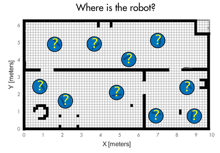
In the previous post, we learnt what is localization and how the localization problem is formulated for robots and other autonomous systems. For the next two posts, we’re going to reference the localization problem that is demonstrated in the MATLAB example, Localize TurtleBot using Monte Carlo Localization. This example simulates a TurtleBot moving around in an office building, taking measurements of the environment, and estimating its location using a particle filter.
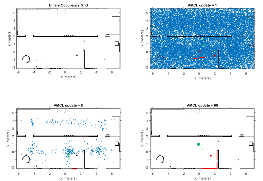
If you’re not familiar with a particle filter it may be confusing as to why the solution has a bunch of blue dots appearing and moving around each time step, and then somehow converging on the real location of the TurtleBot after 60 or so updates. What is the filter doing and how does this seemingly random set of dots help us determine the location of a robot?
To understand how the particle filter solves localization problems, we should develop a little intuition behind the filter with a thought exercise that doesn’t involve robots at all.
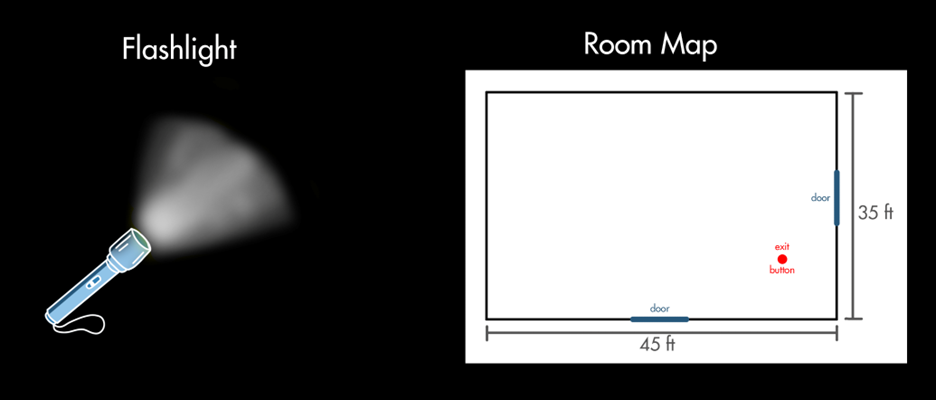
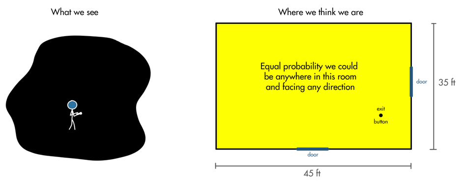
Imagine you wake up in a strange, pitch-black room. You’ve never been in this room before but you’ve been given a map which shows four walls, two locked doors, and the location of a button that opens the doors. You have a small light that allows you to see a few feet in front of you but beyond that it’s total darkness. Our goal is to determine where we are on the map, and then use our location to find the button that will let us out. This is a localization problem.
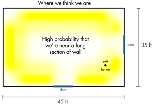
At the beginning, we have no idea where we are in the room. We might say that it is equally probable that we are anywhere on the map and facing any direction.
We turn on our light and we see we are directly facing a wall that is about 3 feet away. From this first observation, can we tell where we are on the map?
Not for sure. There are four walls in this room and we might be facing any one of them, or anywhere along each of the walls. However, we can tell that we are not looking at a corner or the doors, and we are not in the middle of the room since the wall is so close. Knowing that we’re facing a wall at a specific distance away constrains us to one of these positions and orientations.
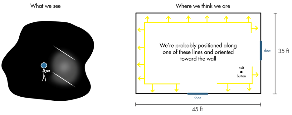
However, since all observations have some amount of noise and error, we might claim that we could be a little closer or further away from the wall than what we are estimating, and we might be slightly turned in one direction or another. Also, we can’t say for sure that we’re not in the middle of the room since it’s possible that we’re looking at a temporary flat obstacle that wasn’t on the map. It’s is a lower probability that that’s the case, but it is still possible so we can’t rule it out.
Therefore, after this first measurement, we may say that the probability distribution of where we are looks something like the image below. With the brighter yellow locations meaning higher probability, and the darker locations lower probability.
This is already a very non-Gaussian probability distribution. Kalman filters require Gaussian probability distributions which is why we can’t use it for this localization scenario. We’ve already failed that constraint with the first observation! A particle filter, on the other hand, does not have that constraint which is why we’re eventually going use it to solve this problem.
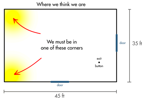
Ok, enough foreshadowing, let’s get back to our thought exercise! Remember, we’re in this pitch black room and all we can see is a wall a few feet in front of us. It makes sense that we can’t be certain where we are from this single measurement, so we need to move around and make another observation. Let’s say we turn to the left and continue to follow the wall for what feels like about 30 feet, eventually reaching a corner. What can we now deduce about where we are currently? We know we’re looking at a corner, so we must be in one of these four areas, right?
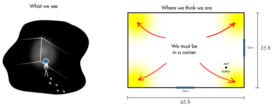
However, we felt like we walked 30 feet, which had to have been almost the entire length of the wall and we didn’t see a door. Therefore, we can rule out the lower right corner and upper right corner as possible locations since we would have had to walk past the door to get to those corners.
This is how we can use our knowledge of past observations along with our knowledge of how we moved to come up with a better estimation of where we are. Our probability distribution now is highest in the two left corners and lower everywhere else. We’re starting to narrow in on our exact location!
Let’s turn once more to the left and keep walking. After about 15 feet we come to a door. Now there are two locations where we could be: facing the bottom door, or facing the right door. However, based on our past observations and our knowledge of how we turned and how far we walked, we can confidently claim that we’re looking at the bottom door. There is only one place on this map where we could turn left, walk 30 feet, then turn left again and walk 15 feet and reach a door.
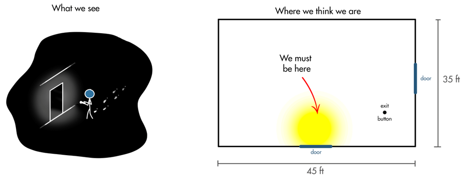
With our location known, we can finally use the map to navigate to the exit button and get out of this crazy room!
As we saw, no single observation was enough to determine our location or pose within the map, however, through successive observations we were able to consolidate where we thought we were into smaller regions, narrowing the probability distribution further until we were confident we knew where we were.
What we did in this example is essentially the same thing a particle filter is doing. If we revisit the TurtleBot example in MATLAB we can start to see how the blue dots represent the possible locations of where the robot is in the office building. As the filter runs, it blends together observations of the environment (sensor measurements) with an estimate of how far the robot travels between measurements and in which direction (motion model) to estimate its location on a map (environment model). Intuitively, this makes sense, right? So, how can we give a robot this ability? How can it remember multiple successive measurements in a way that allows it to hone in on its exact location over time? Well, as we’ve already said, one popular way is with a particle filter, and we’ll talk more about that in the next post.
To learn more on these capabilities, you can watch this detailed video on “Autonomous Navigation, Part 2: Understanding the Particle Filter“. You can also learn more about the Monte Carlo Localization algorithm here. Thanks for sticking around till the end! If you haven’t yet, please Subscribe and Follow this blog to keep getting the updates for the upcoming content.


评论
要发表评论,请点击 此处 登录到您的 MathWorks 帐户或创建一个新帐户。