Sudoku Solver: Image Processing and Deep Learning
This post is from a talk given by Justin Pinkney at a recent MATLAB Expo.
Today’s example will walk through using image processing and deep learning to automatically solve a Sudoku puzzle.
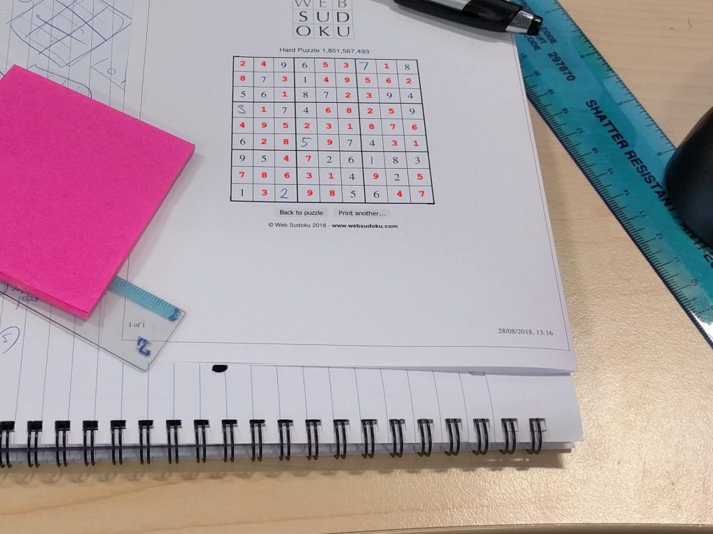 Those red numbers in the puzzle have been automatically added to the paper by the algorithm we're about to create.
This example highlights why deep learning and image processing are both useful for object detection and image classification.
Image Processing and Deep Learning
The two technologies I want to highlight today are:
If you need a refresher on what deep learning is, check out this intro video!
Now, let’s talk about how these two technologies relate to each other. Two common perspectives are:
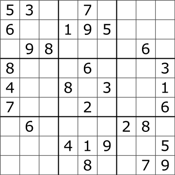 The puzzle begins with some of the numbers filled in. Which numbers and how many are filled in determines the complexity of the puzzle.
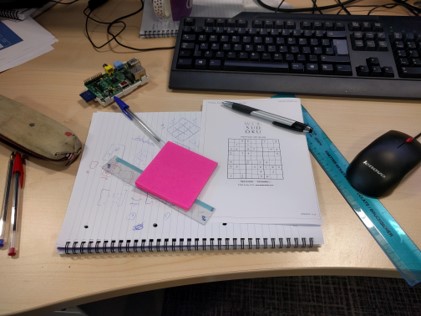
Here, we want our algorithm to find the boxes, and fill in the missing numbers. But that’s almost too easy! We also want to solve the puzzle regardless of where it is in the image. Here’s an example image of where we expect the algorithm to be able to solve the puzzle.
 To solve this, we want to use the right tool for the job, and that means breaking this down into a few distinct parts:
 Here’s the final input data after the it has been labeled.
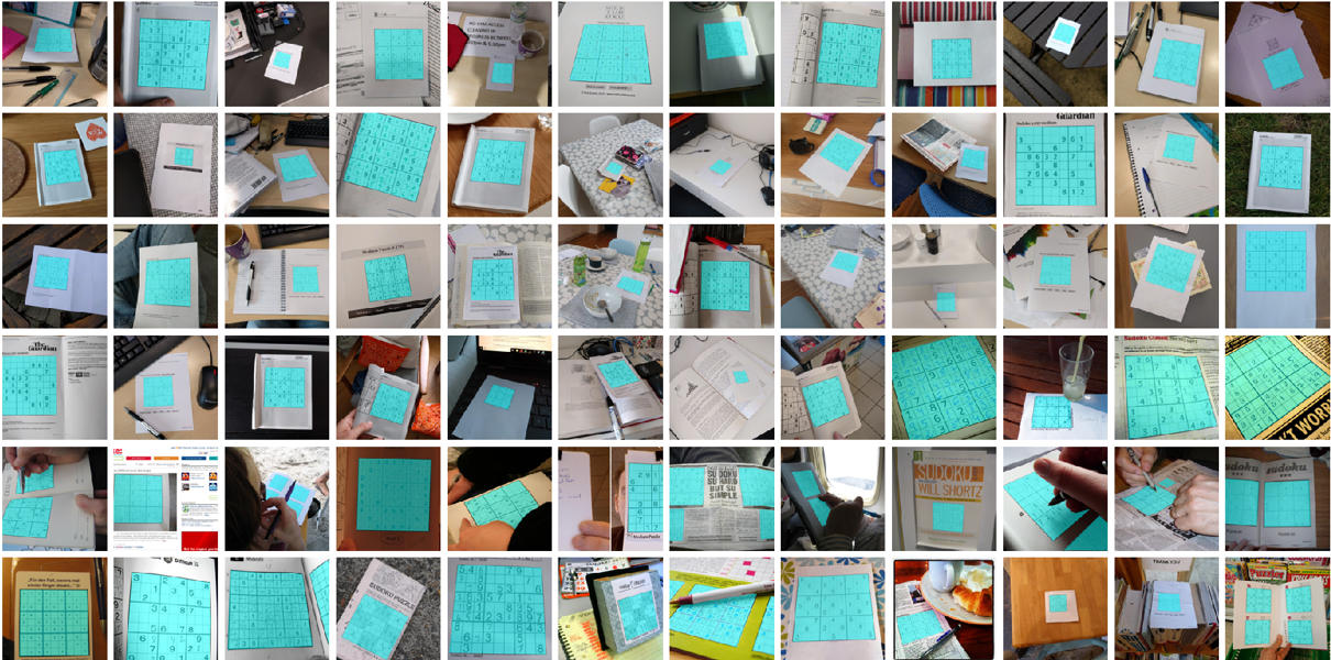 Check out the variability in the training images! Definitely a good deep learning problem. One important thing to note is the dataset is quite small - only around 100 images. Let’s train a semantic segmentation network and see if this data is sufficient.
Setup the image datastores that store pixel information needed for the semantic segmentation network.
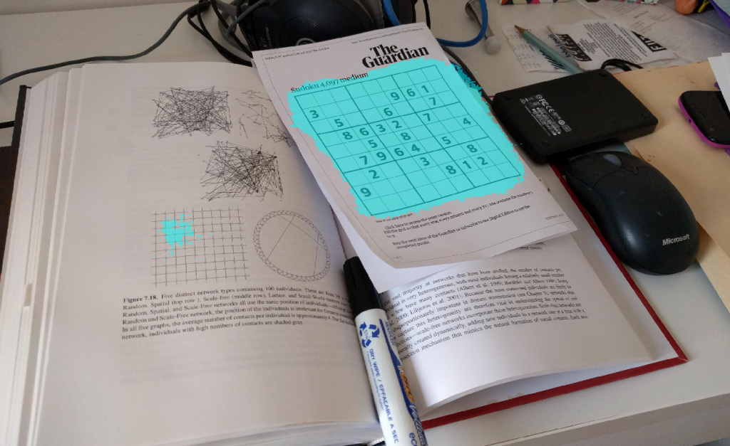 Not bad! It wasn’t even fooled too badly by the other box-shaped figure in the image. The smaller noise can be removed in the next section.
Step 2. Find the Boxes
Here, we need to find the individual boxes in the grid. This is a well-defined problem: straight lines, always dark ink on light paper, and equally sized boxes. Also keep in mind, we already found the approximate location of the box in step 1. We can make everything besides that location black, making this a very cleanly defined problem.
Method? Image Processing
We talk a lot about image processing in our image processing blog. In fact, Steve's blog is the reason I became confident in my image processing skills. The key thing to remember here if you’re not an image processing expert is - you don’t have to be! MATLAB has apps to make this process easy. Check out the Image Segmenter app (here's a video that shows an overview) to explore detecting the boxes in the image. The code below was automatically generated by the app and will detect the individual squares in the image.
First, we have to clean up the image, so any noise is gone.
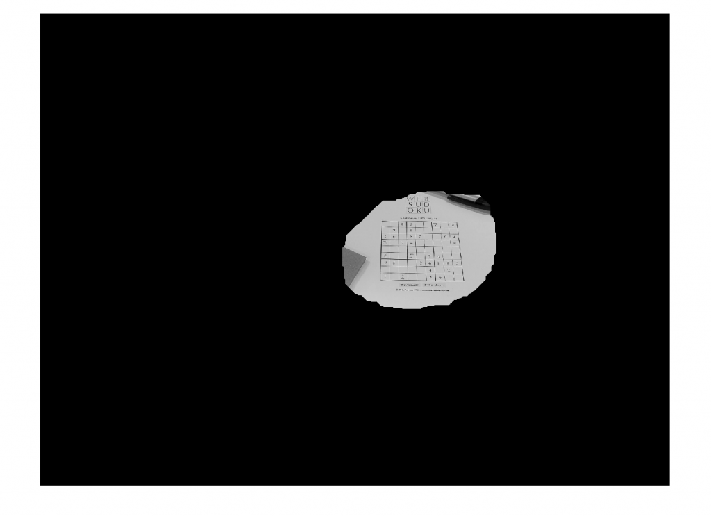 And then find only the box in the image
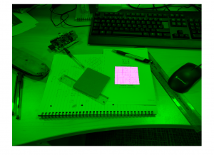 This video shows step 1 and 2 together.
I find these results fascinating... and very robust!
Step 3. Read the Numbers
There are many methods to reading handwritten and typed numbers. This is a challenging problem that must deal with different fonts and styles of numbers, but we have a variety of options:
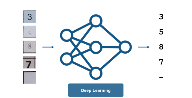 For this, we want lots of training data to account for the different variations in the letters, and when it comes to this much data, we don’t want to be spending hours writing out digits by hand for training.
This is a great opportunity to use MATLAB to generate synthetic data. For the handwritten digits, this is easy – simply steal from the MNIST Dataset and add to our synthetic background shown in the figure below. For creating a variety of typed numbers, we want to vary the numbers to ensure they will be recognized regardless of the font used (Times New Roman, Verdana, etc)
Note: the line widths of the boxes are also made randomly thicker or thinner to account for any discrepancies between boxes.
The idea of synthetic data warrants more time than I can give it in this post. Stay tuned for more posts on this in the future!
We now can train the network. Set the training options, create the layers, and train the network as we did before.
Keep in mind some key tips when tackling a problem dealing with images and video:
 Those red numbers in the puzzle have been automatically added to the paper by the algorithm we're about to create.
This example highlights why deep learning and image processing are both useful for object detection and image classification.
Image Processing and Deep Learning
The two technologies I want to highlight today are:
| Image Processing | Deep learning |
 |
 |
| Transforming or modifying an image at the pixel level. For example, filtering, blurring, de-blurring, and edge detection (to name a few) | Automatically identifying features in an image through learning on sample images. Deep learning has has been revolutionizing the area of image processing in the past few years. |
“Deep learning has made ‘traditional’ image processing obsolete.”or
“Deep learning needs millions of examples and is only good for classifying pictures of cats anyway.”(I’m definitely guilty of classifying a few cats in my day). The reality is:
- Deep learning and image processing are effective tools to solve different problems.
- These tasks are complex: use the right tool for the job.
 The puzzle begins with some of the numbers filled in. Which numbers and how many are filled in determines the complexity of the puzzle.
Here, we want our algorithm to find the boxes, and fill in the missing numbers. But that’s almost too easy! We also want to solve the puzzle regardless of where it is in the image. Here’s an example image of where we expect the algorithm to be able to solve the puzzle.
 To solve this, we want to use the right tool for the job, and that means breaking this down into a few distinct parts:

- Find the Puzzle - locate the box in the image
- Find the Boxes – identify each box of the 9x9 squares
- Read the numbers – these numbers can be digital or handwritten
- Solve the puzzle
 Check out the variability in the training images! Definitely a good deep learning problem. One important thing to note is the dataset is quite small - only around 100 images. Let’s train a semantic segmentation network and see if this data is sufficient.
Setup the image datastores that store pixel information needed for the semantic segmentation network.
train = pixelLabelImageDatastore(imagesTrain, labelsTrain, ...
                                 'OutputSize', inputSize(1:2));
test = pixelLabelImageDatastore(imagesTest, labelsTest, ...
                                'OutputSize', inputSize(1:2));
We can then setup the network layers. It’s interesting to note that Justin made a function to balance the classes using class weighting. Justin pointed out to me that his function does exactly what this example does: https://www.mathworks.com/help/vision/examples/semantic-segmentation-using-deep-learning.html#d120e2892
Setup the network.
numClasses = 2;
baseNetwork = 'vgg16';
layers = segnetLayers(inputSize, numClasses, baseNetwork);
layers = sudoku.weightLossByFrequency(layers, train);
Set up the training options.
    opts = trainingOptions('sgdm', ...
        'InitialLearnRate', 0.005, ...
        'LearnRateDropFactor', 0.1, ...
        'LearnRateDropPeriod', 20, ...
        'LearnRateSchedule', 'piecewise', ...
        'ValidationData', test, ...
        'ValidationPatience', Inf, ...
        'MaxEpochs', 40, ...
        'MiniBatchSize', 2, ...
        'Shuffle', 'every-epoch', ...
        'Plots', 'training-progress', ...
        'CheckpointPath', checkpointPath);
Finally, train the network.
net = trainNetwork(train, layers, opts);This took roughly 20 minutes to run through 40 epochs, though differing hardware/GPUs will produce varying results. On a new test image, we get this result from the trained network:
 Not bad! It wasn’t even fooled too badly by the other box-shaped figure in the image. The smaller noise can be removed in the next section.
Step 2. Find the Boxes
Here, we need to find the individual boxes in the grid. This is a well-defined problem: straight lines, always dark ink on light paper, and equally sized boxes. Also keep in mind, we already found the approximate location of the box in step 1. We can make everything besides that location black, making this a very cleanly defined problem.
Method? Image Processing
We talk a lot about image processing in our image processing blog. In fact, Steve's blog is the reason I became confident in my image processing skills. The key thing to remember here if you’re not an image processing expert is - you don’t have to be! MATLAB has apps to make this process easy. Check out the Image Segmenter app (here's a video that shows an overview) to explore detecting the boxes in the image. The code below was automatically generated by the app and will detect the individual squares in the image.
First, we have to clean up the image, so any noise is gone.
BW_out = bwpropfilt(networkMask, 'Area', [100000 + eps(100000), Inf]);Then we dilate the mask to ensure it covers the entire box.
maskDilated = imdilate(BW_out, strel('disk', 120));
We only care about the location where the box is, zero everything else out
grayIm = rgb2gray(im);
grayIm(~maskDilated) = 0;
 And then find only the box in the image
%% Mask it
BW = imbinarize(grayIm, 'adaptive', 'Sensitivity', 0.700000, 'ForegroundPolarity', 'bright');
% Invert mask
BW = imcomplement(BW);
% Clear borders
BW = imclearborder(BW);
% Fill holes
BW = imfill(BW, 'holes');
imshowpair(im,BW)
 This video shows step 1 and 2 together.
I find these results fascinating... and very robust!
Step 3. Read the Numbers
There are many methods to reading handwritten and typed numbers. This is a challenging problem that must deal with different fonts and styles of numbers, but we have a variety of options:
- Optical character recognition (OCR) is a common method
- HOG with a machine learning classifier is another option. A MATLAB example is here
 For this, we want lots of training data to account for the different variations in the letters, and when it comes to this much data, we don’t want to be spending hours writing out digits by hand for training.
This is a great opportunity to use MATLAB to generate synthetic data. For the handwritten digits, this is easy – simply steal from the MNIST Dataset and add to our synthetic background shown in the figure below. For creating a variety of typed numbers, we want to vary the numbers to ensure they will be recognized regardless of the font used (Times New Roman, Verdana, etc)

resolution = size(im, 1);
maxSize = resolution - 2*border;
fontSize = round((maxSize - minSize)*rand(1) + minSize);

textColour = maxColour*rand(1, 3);
position = [resolution/2, resolution/2] + maxOffset.*(rand(1, 2) - 0.5);
For both types of synthetically generated numbers, we want to vary the size and location of the numbers. This is what allows us to generate as much data as we want!

|

|
| Synthetic Image - Handwritten | Synthetic Image - Typed |
options = trainingOptions('sgdm', ...
                          'Plots', 'training-progress', ...
                          'L2Regularization', 1e-2, ...
                          'MaxEpochs', 8, ...
                          'Shuffle', 'every-epoch', ...
                          'InitialLearnRate', 0.01, ...
                          'LearnRateDropFactor', 0.1, ...
                          'LearnRateDropPeriod', 3, ...
                          'LearnRateSchedule', 'piecewise', ...
                          'ValidationData', test, ...
                          'ValidationPatience', Inf, ...
                          'MiniBatchSize', 64);

% This is creating a network from scratch that closely resembles VGG16
layers = sudoku.training.vggLike(initialChannels, imageSize);

% Train
net = trainNetwork(train, layers, options);
For this example, it’s looking like the network is getting roughly 97.8% accuracy. That accuracy is sufficient... for a Sudoku solution.
Step 4. Solve the Puzzle
We have the boxes and the numbers. Now we need to fill in the other values.
Method? Neither! This is an optimization problem
We’ve written about Sudoku solvers previously:
- Cleve’s post on Sudoku is here: https://www.mathworks.com/company/newsletters/articles/solving-sudoku-with-matlab.html
- Or check out the optimization code in this documentation example: https://www.mathworks.com/help/optim/examples/solve-sudoku-puzzles-via-integer-programming.html
 |
 |
 |
 |
 |
 |
 |
 |
- Deep learning is sometimes, but not always, the right tool for the job
- Both image processing and deep learning are great tools that can be combined to form the right solution You can download the complete solution here: https://www.mathworks.com/matlabcentral/fileexchange/68980-deep-sudoku-solver, and leave a comment for Justin below if you have any questions.
- カテゴリ:
- Deep Learning


コメント
コメントを残すには、ここ をクリックして MathWorks アカウントにサインインするか新しい MathWorks アカウントを作成します。