
How Do We Know Our System Will Actually Work?
I talk about Model-Based Design a lot and in different forums: industries, universities, conferences. I usually position it as a way of ensuring our systems behave as we intended them to.
And almost every time, someone asks the obvious follow-up (paraphrasing a bit): how do I actually know the system behaves the way I intended?
Then I’ll normally talk about V&V, testing under different conditions, checking your system at different stages of its lifecycle. All of which is true, mind you, albeit fairly abstract. If you already know the answer, it all makes sense. If you don’t, it probably sounds like engineering word-salad.
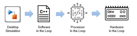
So, in this blog, let’s talk about: desktop simulation (which is sometimes referred to as Model-in-the-Loop (MiL)), Software-in-the-Loop (SiL), Processor-in-the-Loop (PiL), Hardware-in-the-Loop (HiL). What each one actually means, when you’d reach for each, and why it matters.
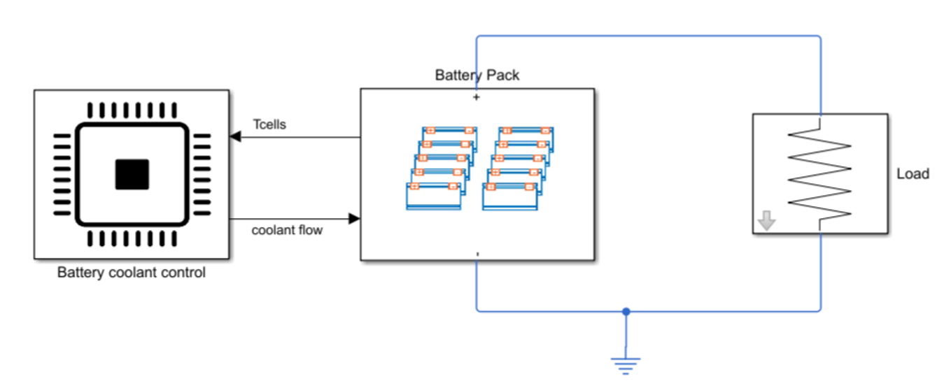
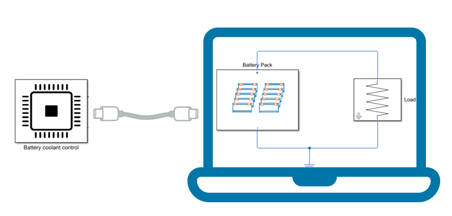
Let’s look at the temperature control of a battery pack as an example. In this abstracted Simulink block diagram, we have a battery pack (our plant), the load it is driving and a controller that takes in the measured temperature of the pack and provides the appropriate coolant flow. The cooling system is integrated inside the battery pack subsystem.
Desktop Simulation 
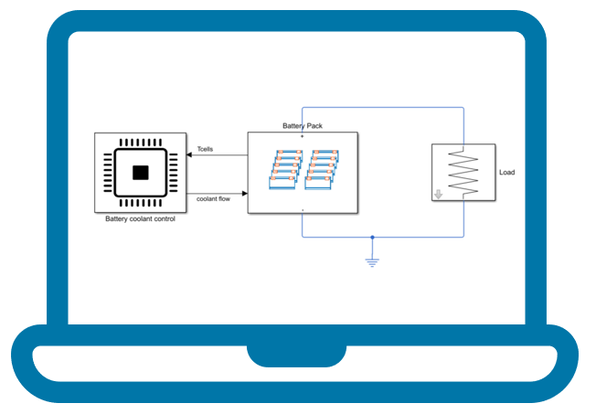
This is the easy one… I mean, if you’re here you probably use Simulink, MATLAB or some other tool to model your systems, right? If so, you’ve done it! You’ve modeled your algorithms before you put them on your real system. Here, everything runs in simulation, our controller, our pack, our load, they’re all in Simulink and Simscape.
Why start with simulating on our desktop? Later stages let you see signals and change things too, but here is where we can do it in isolation. Nothing is constrained by generated code, a target processor or real-time deadlines yet, we are free to focus on the design itself, the control law and the plant dynamics. That isolation is what lets us iterate fastest: change anything and explore the solution space freely. If the loop is unstable, if the controller chatters around the setpoint, if our fallback logic doesn’t trigger when a sensor drops out… we can find that out *here*, cheaply, before any hardware constraints cloud the picture.
For our battery pack, this is where we can confirm that the coolant flow controller actually holds the pack temperature at setpoint across a realistic profile; or that it fails gracefully if the temperature sensor drops. This is where we’d also explore different failure modes safely.
Software in the Loop (SiL) 
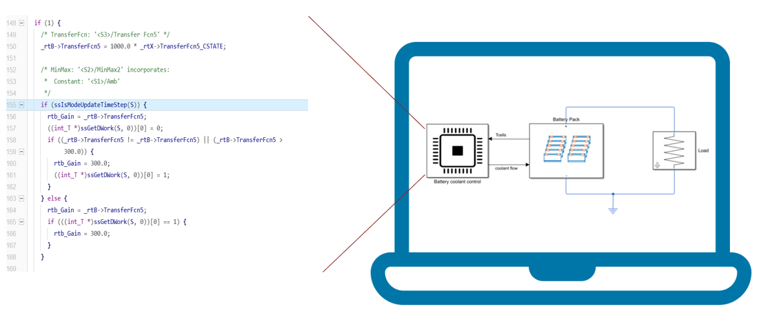
Now generate C from the controller model, compile that generated code for our development machine, and run it against the same plant model. The controller is now the actual software we intend to run on our device (not a Simulink representation of it).
Architecturally, not much changes from our desktop simulation: the same test harness drives the same plant model, and we simply swap the Simulink subsystem that held the controller for a block that runs the generated C code instead.
In my case, this translation from Simulink to C has never been manual. I tend to use tools like Embedded Coder to facilitate that and ensure full traceability of each line of C back to my model’s blocks.
Why do SiL? Why compare our C to our Simulink response? It allows us to check if the implementation that is going to our embedded hardware matches our Simulink design. This allows us to check for any effect on precision/ data type conversion/ quantization errors. We could also check the possible implementations for different hardware.
Again, everything happens on our host machine. But, instead of Simulink, our controller now runs the C code that will go on our hardware (soon!).
Processor in the Loop (PiL)
Now if we are happy that our embedded code matches our design, the next step is to test it on the actual board. Here, the algorithms live on the board, but our plant still lives in simulation.
Why do we want to do PiL? we want to check if the target executes the code reliably and if it produces the same answers as the host. This is where we may find out that the sample rate you assumed at the desktop simulation stage was optimistic.
Also, processors differ in word length, floating-point support, memory hierarchy, and interrupt behavior. Code that comfortably held its sample rate on our desktop may not on a small embedded part.
For our battery pack, this is where we’d confirm the controller keeps its thermal sample rate on the actual board and the flow rate it computes matches what the host produced.
One caveat: PiL is not (necessarily) real-time. The board and the host exchange data step by step, and the plant, still simulating on the host, simply waits for the board between steps. That makes it a cross-target, co-simulation kind of test, and testing can get slow when the host-side model is heavy. So, the questions we are trying to answer here are mostly functional, rather than temporal.
Hardware in the Loop (HiL) 
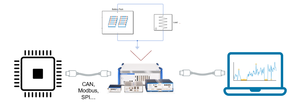
Now the plant model moves onto a real-time simulator, for example a Speedgoat system, running in hard real time on hardware built for deterministic execution, and the controller talks to it through its own physical I/O.
At the system level, the controller no longer sees simulated numbers handed to it on the host’s schedule; it exchanges signals with a plant that is always running and always presenting values for it to react to, on the same kind of interfaces it will meet in the field. Those interfaces are real: analogue channels carrying real voltages, PWM outputs driving a real actuator signal, and CAN, SPI or Modbus traffic arriving over the wire, when it arrives.
Worth noting from a workflow point of view: even though the plant has left the host computer, from the user’s side little changes. The Simulink model on our computer becomes a console onto the target, and we start, stop, tune and log the model running on the real-time hardware much as we would a model running locally. The host is now doing the monitoring and analytics, and the real-time computation is happening on the target.
What’s the question HiL attempts to answer?
Our algorithm can be right, our code faithful and our processor fast enough, and the loop can still behave differently once every signal path is real. The controller is not waiting for anything; the plant is simply running, and the controller has to react to signals as they actually arrive, with the real timing, delays and jitter of physical interfaces rather than the instantaneous, perfectly ordered exchange it saw at every earlier stage. For our battery pack, HiL is where we’d find out whether the controller still holds pack temperature once it’s the real board driving real outputs, with the actual latency of sensor and comms traffic between the pack and the controller, rather than the instantaneous, perfectly ordered exchange every earlier stage assumed.
Something to keep in mind, HiL needs a real-time plant simulator and matching I/O hardware, which is a genuine capability threshold rather than a line item. How far we can get without it depends heavily on the dynamics. For slow, latency-tolerant systems like the thermal loop in this example, PiL may well be far enough for a research prototype. For fast, latency-sensitive plants, a motor drive being the obvious case, the host will never simulate quickly enough to close the loop, and PiL stops being sufficient long before we reach production.
What checks what
- Desktop Simulation (MiL) checks the algorithms against the system architecture.
- Software in the Loop (SiL) checks the generated code against the algorithms.
- Processor in the Loop (PiL) checks the target performance against the code.
- Hardware in the Loop (HiL) checks the integrated unit against the requirements.
Worth mentioning that when one of these fails, it is worth identifying what we were testing before “fixing” that stage. Timing missed at PiL: underspecified processor, or an algorithm doing more than it needs to? Drift at SiL: wrong datatype, or model design leaning on precision it was never going to get?
This, for me, is part of the appeal of Model-Based Design. The models and test harnesses and scenarios you build for desktop simulation aren’t throwaway. We get to reuse the same ones for SiL, PiL, and HiL, so you’re checking each stage against a consistent set of conditions rather than rebuilding your tests four times. And because the outputs are all logged the same way, you can line up results from desktop simulation, SiL, PiL, and HiL directly in the Simulation Data Inspector to see exactly where and when two stages diverge, which is what turns “the board doesn’t match the host” from a vague worry into a specific signal at a specific timestep.
So, how do you know your system will actually work?
By doing all of these, you reduce the risk of your prototype failing and that matters more the more expensive or safety-critical the thing you’re building is.
Which is really what decides how far up the ladder you go. For a research prototype, MiL and SiL with PiL once the target gets involved is probably sufficient. For something heading into production, all four are standard, and in safety critical and regulated domains they underpin certification frameworks like ISO 26262 and DO-178.
Beyond that there’s more still: virtual ECU testing, multi-node HiL, power HiL where real power electronics are in the loop.
Further reading & resources
- Test Generated Code with SiL and PiL Simulations – for going deeper on SiL and PiL workflows and testing equivalence between model and generated code
- Simulink Real Time (for HiL and RCP)– for running your plant model in hard real time on Speedgoat target hardware
- Simulink Coder, Embedded Coder, GPU Coder, HDL Coder – code generation tools to produce C/C++, CUDA and HDL code
- Model-Based Design for DO-178B – how this maps onto avionics certification.


See Also
-

It's Time for Real-Time!
Blogs
-
-
-

コメント
コメントを残すには、ここ をクリックして MathWorks アカウントにサインインするか新しい MathWorks アカウントを作成します。