Guest writers: Mohan Parthasarathy and Padmanabhan Seshaiyer, PhD Mohan Parthasarathy is a student at Thomas Jefferson High School for Science and Technology. Padmanabhan Seshaiyer, PhD, is Professor of Mathematics at George Mason University.

In this blog post, we discuss PINNLab, an interactive MATLAB application for exploring parameter estimation in differential equation models using physics-informed neural networks (PINNs).

Many scientific and engineering problems require working backward from limited observations to understand the system that produced them. Suppose you know the equations governing a population, an epidemic, or a chemical process, but not the growth rate, transmission rate, or reaction constant. Given a small collection of noisy measurements, how can you recover those missing parameters?

This is an inverse problem: working backward from observations to infer the parameters that produced them. We built PINNLab to make that process interactive. Users choose a model, provide observations, train a physics-informed neural network, and examine whether it recovers both the system trajectory and its hidden parameters.

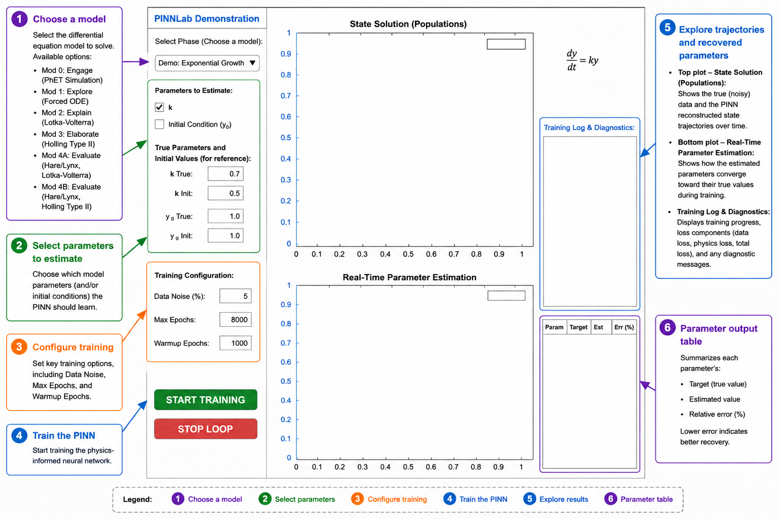
Figure 1. The PINNLab interface for configuring and solving inverse problems.

A standard neural network learns by fitting observed data. A physics-informed neural network, or PINN, learns from both the data and the governing equations describing the system.

For an ODE, the network approximates the system state x(t), while automatic differentiation provides its derivative. Training balances data fit, the differential equation residual, and the initial conditions, while estimating the unknown parameters θ.

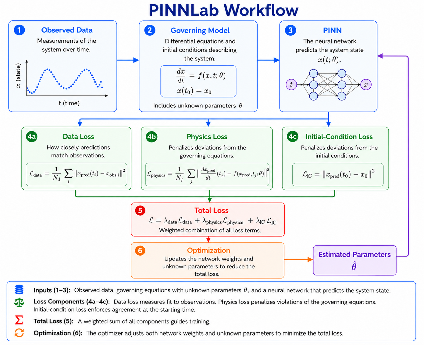
Figure 2. How a PINN combines data and governing equations during training.

This does not mean PINNs replace numerical methods. Conventional optimization may be faster for small, well-identified models. PINNs become especially interesting when data are sparse, some states are hidden, or states and parameters must be reconstructed together. PINNLab helps users explore that tradeoff rather than assume the PINN will always win.

Most differential equations courses focus on forward problems: you are given the equation and parameters, and your job is to solve for the state.

Research rarely works that way. More often, you have the equations and data, but the parameters are exactly what you are trying to discover. That drew us to inverse problems and, eventually, PINNs.

As we experimented, we kept rebuilding the same pieces: physics residuals, custom training loops, trajectory plots, and parameter comparisons. Many examples we encountered were research-oriented Python implementations: useful for reproducing results, but not designed for students to change assumptions and see why the model behaved as it did. Eventually we realized something had changed. We were not just building models anymore; we were building a learning environment, one we found equally useful for rapidly prototyping and testing inverse problem workflows during research.

PINNLab grew from the questions that kept coming up: Where does the network get its information? What happens when data become sparse? When does the differential equation help? MATLAB gave us a natural way to bring those questions into one place. Deep Learning Toolbox handles automatic differentiation and custom training, while App Designer puts the mathematics, controls, and visual feedback into an interactive app.

PINNLab follows the 5E instructional framework: Engage, Explore, Explain, Elaborate, and Evaluate. Learners begin with a scientific question, experiment with a simpler system, and gradually build the mathematics needed to address it.

We also drew on the U.S. Department of Labor's AI Literacy Framework, which emphasizes understanding what AI can and cannot do, evaluating its outputs, and keeping human judgment central. In PINNLab, learners do more than click Train: they are encouraged to experiment. What happens if you remove half the observations? What if you estimate six parameters instead of two? What if the governing equation is slightly wrong? PINNLab lets users change those assumptions and immediately see how the trajectories, residuals, and parameter estimates respond. The goal is not simply a low loss, but an understanding of why the model succeeded or failed.

In that sense, PINNLab becomes more than a PINN implementation. It is a place to see how inverse problems behave, making machine learning more accessible and helping users develop the judgment needed to apply AI responsibly in scientific work.

PINNLab's current curriculum follows an ecological storyline centered on Canadian snowshoe hares and lynx. Open the app, choose the Lotka-Volterra predator-prey model, select which parameters the network should learn, and import or generate observations. When you click Train, the PINN reconstructs both populations while estimating the ecological parameters.

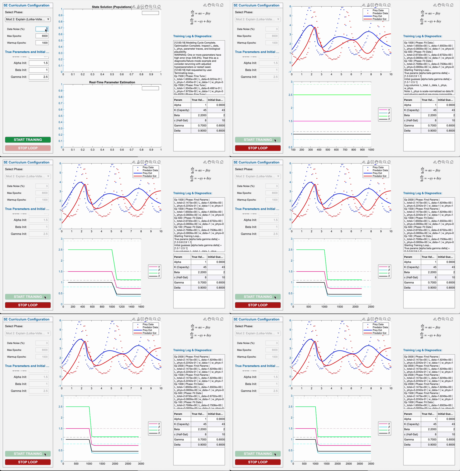
Figure 3. Exploring parameter estimation by changing observations and retraining the PINN.

During training, the network weights and ecological parameters are optimized simultaneously. Once training finishes, PINNLab reports the recovered parameter values alongside their initial guesses and, when the true values are known, their relative errors. The curriculum then introduces logistic prey growth and a Holling Type II functional response, creating a six-parameter inverse problem.

The table below shows one result for the Holling Type II model.

Table 1. Recovered parameter estimates for the logistic-growth Holling Type II predator-prey model.

The estimates recover the overall parameter scale, although some parameters are identified more accurately than others. Differences like these help learners see that parameter recovery depends not only on training performance, but also on how strongly each parameter is identified by the available observations.

The six-parameter inverse problem raises a natural question: How many parameters can a PINN estimate at once? There is no universal answer. It depends on the information in the data, parameter identifiability, and model quality. In several PINNLab experiments, we were able to estimate as many as eight unknown parameters, although accuracy depended heavily on the model and data. But as the number increased, the problem quickly became one of identifiability, not just computation. That is exactly what we want learners to discover.

Finally, learners upload historical Hudson's Bay Company hare-lynx records and compare competing models against real data.

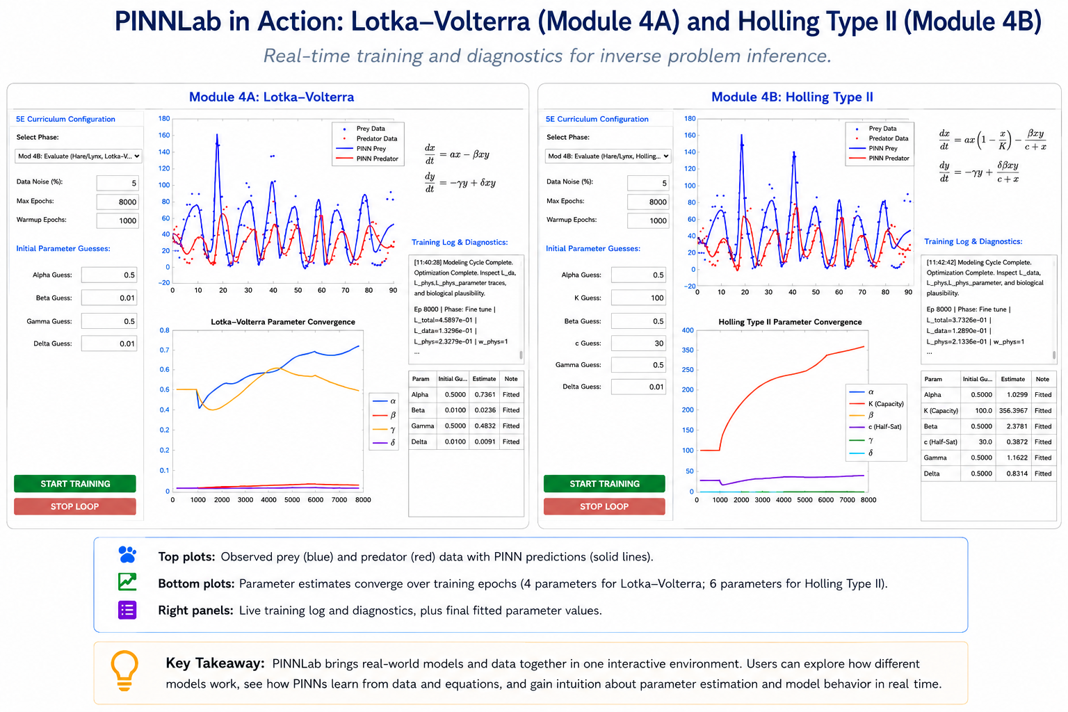
Figure 4. Comparing competing predator-prey models using historical hare-lynx observations.

Before building PINNLab, we assumed that if a network reproduced the observed data, it must also have learned the correct parameters. Inverse problems taught us otherwise: an accurate-looking trajectory does not guarantee accurate parameters.

A network may fit the observations while compensating for an incorrect parameter elsewhere in the model. Conversely, a physics residual that refuses to converge may reveal that the governing equation itself is inconsistent with the data.

That is not necessarily an algorithmic failure. It may be evidence that the model needs to change.

This distinction between fitting data and validating a scientific explanation became one of PINNLab's most valuable teaching features.

Once PINNLab worked well for ecology, the next question was: Where else can this idea go? We are now expanding the platform toward disease dynamics, contaminant transport, hemodynamics, and pharmacological modeling. We are also interested in exploring how PINNs fit within the broader modeling ecosystem, including established parameter-estimation workflows such as those available in SimBiology.

We are in the process of adding guided modules, stronger diagnostics, and support for more complex parameters. Our goal is not to make every problem look like a PINN problem, but to help users recognize when physics-informed learning adds value.

We built PINNLab because inverse problems deserve the same kind of interactive learning environments that already exist for solving differential equations. Physics-informed neural networks can combine mathematical models with observational data, but understanding when they work is just as important as knowing how to run them.

We hope PINNLab gives you a place not only to train a PINN, but to ask the more important questions: What did the network actually learn? Why should you trust it? And what does the governing equation contribute that the data alone cannot?

Let us know in the comments what kinds of inverse problems you'd most like to explore with PINNLab. Check out the open-source PINNLab code and examples on GitHub and read our accompanying CODEE Journal article.