
Casting Shadows and Inverse Stereographic Projections
 |
Guest Writer: Eric Ludlam Joining us again is Eric Ludlam, development manager of the MATLAB charting team. Discover more about Eric on our contributors page. |
In the previous blog article, we talked about how to simulate simple shadows in MATLAB. Given a light source and a shape, we were able to draw some convincing shadows on the floor of the axes. But what if you have a shadow, and you want to compute a shape that can cast it?
One way to do that is to use a stereographic projection which lets you project vertices between a sphere and a flat surface. Map makers have been transforming features on the earth into flat maps for a long time. Mapping toolbox's new mapaxes (R2023a) lets you explore several kinds of projections. Here's an example of a stereographic projection using mapaxes.
% If you don't have Mapping Toolbox, you can skip this example
prj=projcrs(53026,'Authority','ESRI');
prj.ProjectionParameters.LatitudeOfNaturalOrigin=90;
newmap(prj)
land=readgeotable("landareas.shp");
land(land.Name == "Antarctica",:) = [];
geoplot(land)
geolimits([30 90],[-180 180])
title('Stereographic Projection')

In this projection, the north pole of the earth (the top part of the sphere) is being projected onto a plane (your screen). Mapping toolbox projections cover a wide range of interesting options. We can use similar techniques as Mapping toolbox to project our 2D pattern in the opposite direction, back onto a sphere.
So with that background, let's pick out a shape we want as our eventual shadow. A hex-grid will be a good shape to use, because it looks neat when projected onto a sphere. I have a helper function I'll call here which returns a Polyshape object.
ps = hexgrid; % see end of this live script
plot(ps)
axis equal

As shadows go, this will be pretty interesting. Next, we need to get our vertices out of the Polyshape object. We'll convert it into a triangulation, as the triangulation tools have handy features, we can take advantage of.
psTri = ps.triangulation();
pts = psTri.Points;
faces = psTri.ConnectivityList();
We now need to do a reverse projection onto a sphere using a north pole stereographic projection similar to what we saw in the Mapping toolbox example. This projection will use a large portion of the sphere based on size of the polyshape we made. We only need to project the points, as the connectivity will remain the same between the desired shadow, and our new shape. This optimization works because the shadow fits wholly on the sphere.
Starting with the shadow points in pts, we can project onto a unit sphere (radius==1) which we assign to SpherePts. In the following code, X and Y are column vectors. The result is a Nx3 matrix whose columns are X, Y, and Z respectively that specify the projection of the shadow onto the 3D sphere.
X=pts(:,1)/2;
Y=pts(:,2)/2;
H=X.^2+Y.^2;
SpherePts = [ 2*X./(H+1), 2*Y./(H+1), (H-1)./(H+1)+1 ];
Now that we have the points on the sphere, we'll use the new vertices and the original faces array to create a triangulation. The triangulation is nice because it will give us access to the freeBoundary function, which enables us to draw the outer boundary of the shape without the internal triangulation.
The code below creates 2 patches, one to draw the blue part (the full stereographic projection of the shadow onto the sphere), and the second draws the "edge" of the shape. That edge adds some artistic definition where parts of the shape overlap each other in the below view.
Tri = triangulation(faces, SpherePts);
newplot
patch('Vertices',Tri.Points,'Faces',Tri.ConnectivityList(),...
'FaceColor',lines(1),'EdgeColor','none');
patch('Vertices',Tri.Points,'Faces',Tri.freeBoundary(),...
'FaceColor','none','EdgeColor','black');
view(3)
axis equal padded
grid on

Since we're talking about shadows, let's add a light just over the "north pole" of our sphere and we'll drop a marker where the light is to make it easier to reason on what you see. Setting the light object's 'Style' property to 'local' makes the light emit in all directions. In the image below, this means it looks like the light is shining from inside the sphere, and not on the outside.
Lpos=[0 0 2];
light('Position',Lpos,'Style','local');
Lm=line(Lpos(1),Lpos(2),Lpos(3),'Color','red',...
'Marker','o','MarkerFaceColor','auto',...
'MarkerSize',10,'LineWidth',1);
lighting gouraud
material([ .6 .9 .3 2 .5 ])

Lastly, we'll pull our code-snippet for drawing shadows from the previous article and use it on our newly created shape.
pts = Tri.Points;
shadowPts = zeros(size(pts));
shadowPts(:,1:2) = Lpos(3).*(pts(:,1:2)-Lpos(1:2))./(Lpos(3)-pts(:,3))+Lpos(1:2);
Ps = patch('Vertices',shadowPts,'Faces', Tri.ConnectivityList,...
'FaceColor', [.6 .6 .6], 'FaceAlpha', .5, 'FaceLighting','none',...
'EdgeColor', 'none');

In the above image, we have the stereographic projection of our original polyshape, a light object to illuminate it, and we then re-cast the shadow back onto the floor of the axes, showing that our projection worked!
I took this shape and wrote some additional code to turn it into an STL file that you can 3D print. Thanks to MathWorker Eric Felton for 3D printing the shape pictured below for this blog article!

In the above image, a small flashlight was used to cast a shadow of the 3D printed shape into a countertop.
You can download the Shadows for MATLAB project from github or File Exchange to get all the code for this blog in handy utility functions, plus a repository of STL files you can print for different stereographically projected shapes. This File Exchange project includes additional shadow casting features, such as a function that will let you create shadows on all the axes walls: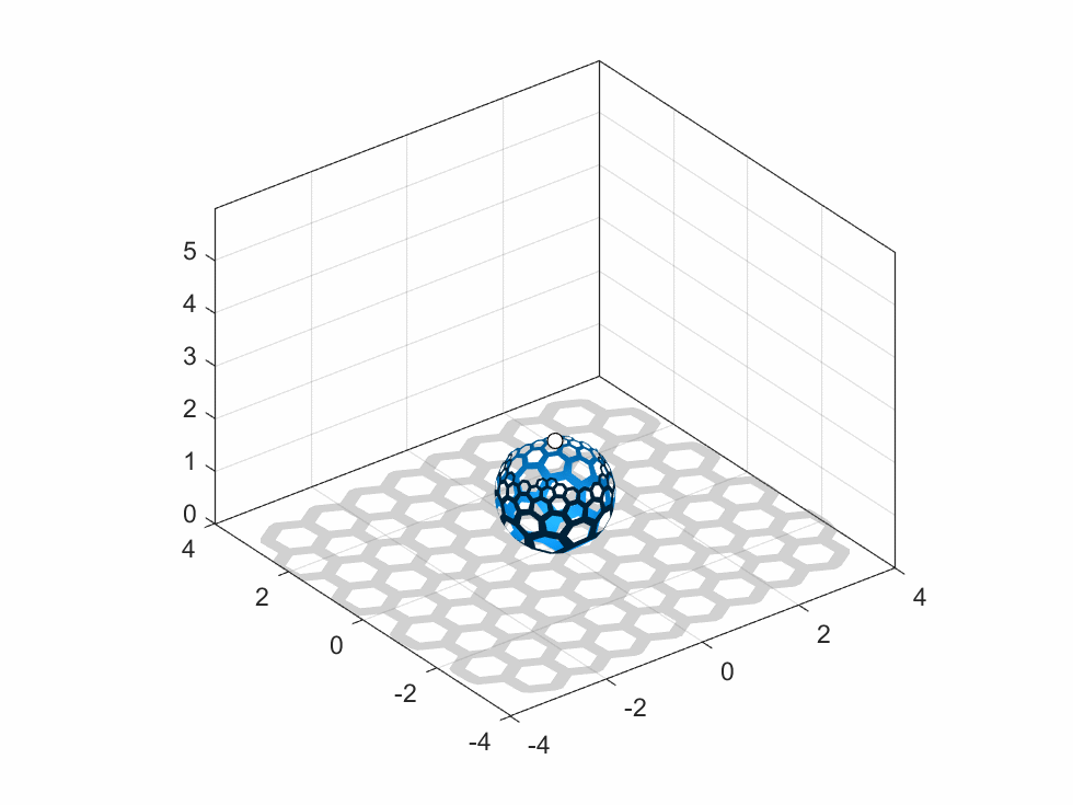
function ps=hexgrid
% Compute a hexgrid polyshape with evenly wide edge lines.
R=.5; row = 9; col = 8;
theta=linspace(0,2,7);
xhex=sinpi(theta)*R;
yhex=cospi(theta)*R;
D=cosd(30)*R;
ps=polyshape.empty();
WIDTH=col*D*2;
HEIGHT=(row-1)*R*1.5;
for i=1:(col+1)
j=i-1;
for k=1:row
if i<=col || ~mod(k,2)
m=k-1;
xbuff = ((xhex+mod(k,2)*D)+D*2*j)'-WIDTH/2;
ybuff = (yhex+1.5*R*m)'-HEIGHT/2;
ps(end+1) = polybuffer([xbuff ybuff], 'lines', R/4); %#ok
end
end
end
ps=union(ps);
end


댓글
댓글을 남기려면 링크 를 클릭하여 MathWorks 계정에 로그인하거나 계정을 새로 만드십시오.