At multi-gigabit data rates, a clean-looking channel simulation can still leave you with a failing eye. The hard part is not just measuring that jitter exists; it is figuring out which timing effects are closing the eye, how much margin they are consuming, and whether the next design move should be clock cleanup, equalization, channel modeling, or noise reduction.

This article shows how to turn total jitter from a single pass/fail number into design guidance. We’ll walk through two practical workflows: one for controlled waveform experiments where impairments can be injected and checked, and one for observing jitter metrics directly inside a SerDes system simulation as the design runs.

Along the way, we’ll separate random, deterministic, sinusoidal, duty-cycle, and ISI-related jitter; show where the estimates are reliable or fragile; and close with a checklist for getting numbers you can trust before making design decisions.

Interested to learn more? visit our MathWorks Solutions for Semiconductors Site

From Total Jitter to Actionable Components

In practice, jitter is rarely a single phenomenon. What you typically care about is shown in Figure 1 and defined below.

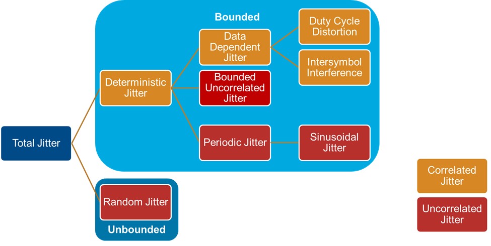
Figure 1: Breakdown of Jitter into the various types

 

• Total jitter (TJ): what the receiver “feels” at the sampling instant
• Random jitter (RJ): unbounded, unpredictable timing deviation
• Deterministic jitter (DJ): bounded timing variation that includes periodic and data-dependent effects
• Data-dependent jitter (DDJ): deterministic jitter correlated with the transmitted data pattern, often caused by duty-cycle distortion and intersymbol interference
• Duty-cycle distortion (DCD): systematic even/odd or rise/fall timing asymmetry
• Intersymbol Interference (ISI): channel dispersion causing overlapping signal pulses between adjacent symbols
• Periodic jitter (PJ): bounded deterministic jitter that repeats at one or more specific frequencies
• Sinusoidal jitter (SJ): periodic jitter with identifiable frequency content

One way to group jitter is by whether it’s bounded or unbounded. Bounded jitter has upper and lower amplitudes while unbounded jitter, theoretically, does not.

Another way to group jitter is whether it’s correlated or uncorrelated. Correlated jitter is connected to the data pattern itself while uncorrelated jitter is not connected to the data pattern. It comes from something unrelated to the data pattern, like a clock, crosstalk, or thermal noise.

These distinctions matter because modern measurement workflows can exploit them by turning total jitter from a single number into a set of actionable diagnostics.

A measurement approach that separates these components helps you answer the questions that matter in bring-up and architecture work. For example:

• Is the “extra” jitter coming from noise-like effects, such as RJ, or from a bounded deterministic source, such as SJ, PJ, DCD, DDJ, or from crosstalk?

• Is one symbol interfering with the next through ISI, meaning you should focus on equalization and channel modeling first?

Jitter degrades the eye diagram regardless of its source, as illustrated in Figure 2. The eye diagram on the left represents a system without any extra Tx or Rx jitter added and shows an eye width of 79.6 ps. In contrast, the eye diagram on the right corresponds to the same system with some RJ and DJ jitter added, where the eye width decreases to 63.5 ps, a ~20% reduction.

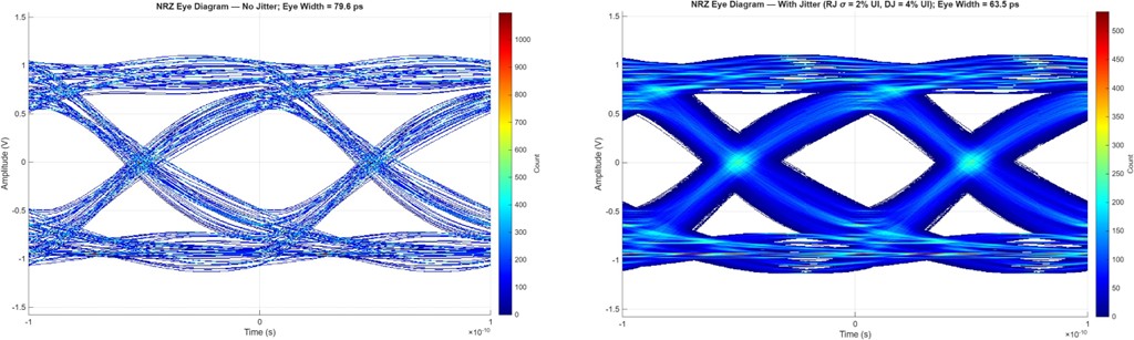
Figure 2: Left – eye diagram with no Tx or Rx jitter and eye width = 79.6 ps. Right – eye diagram with jitter and eye width = 63.5 ps

 

Once the eye is closing due to jitter, the next question is which jitter sources are responsible.

Two Workflows, One Goal

Waveform-based workflow: Inject impairments, estimate jitter components, sanity-check results

The first example focuses on a simple but powerful loop: generate a waveform –> add jitter impairments –> measure timing error –> estimate jitter components.

At a high level, the workflow looks like this:

1. Create an oversampled stimulus (for example, a PRBS pattern at a chosen unit interval).
2. Apply jitter impairments such as DCD, SJ (with frequency), and RJ to the stimulus configuration.
3. Generate the waveform.
4. Measure jitter metrics.

Here’s the key value: the estimate returns both TJ metrics and component estimates (RJrms, DJpkpk, SJa/SJf/SJp, DCDpkpk, and more).

Why this is useful: it’s easy to sanity-check the setup by comparing the injected impairments with the estimated results, such as verifying how DCD is represented and how SJ amplitude maps to the estimate. It also makes it straightforward to inspect the timing interval error and see how the jitter components relate, with Figure 3 showing how the workflow leads to those results.

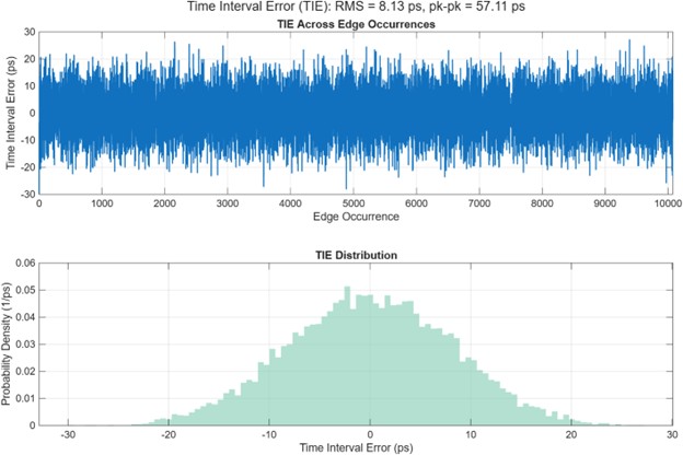
Figure 3: Timing Interval Error Edge Occurrences and Distribution

Time Interval Error (TIE) is a measure of how each event’s timing in a signal deviates from its ideal schedule. In practice, it indicates whether each successive clock cycle or data interval arrives slightly early or late relative to a perfect reference, effectively capturing the accumulated timing jitter over time.

Also, Timing Error (TE) is the difference between the measured signal transition time and the ideal transition time defined by the reference symbol clock. Evaluated across many unit intervals, the resulting timing error captures the combined effects of random, deterministic, and data-dependent jitter components.

Do not skip this: Accuracy vs precision in component estimates

Not all jitter metrics should be trusted equally without context. One of the most practical takeaways from the waveform-based example is that different jitter metrics behave differently in terms of accuracy and sensitivity to measurement assumptions.

• TJ metrics are computed directly from the TE sequence, so if edge detection and alignment are correct, TJ tends to be accurate.
• RJ RMS is commonly overestimated, because it is effectively “what is left” after subtracting other component estimates from the TE. Any error in other components leaks into RJ.
• DJ and DDJ are combinations of other jitter metrics (DDJ = DCD + ISI and DJ = DDJ + SJ).
• SJ estimates depend on a discrete Fourier Transform (DFT)-based approach; frequency-bin alignment affects accuracy, and phase can be particularly sensitive.

Measuring ISI-related jitter: consider supplying an impulse response

Estimating ISI-related jitter typically involves recovering a pulse/impulse response from the data, then synthesizing an “ISI-only” waveform for timing error comparison.

That recovery can be distorted if the waveform also contains significant non-ISI jitter. A practical remedy is to provide an impulse response directly (from a simulated channel model, extracted channel response, or a fitted model), which improves the stability of the ISI characterization.

In-model workflow: View jitter metrics as the SerDes simulation runs

If waveform-based analysis tells you what happened after a run, in-model measurement helps you see when it happens. This workflow places a jitter measurement stage in the data path of a time-domain SerDes simulation, so timing error and component metrics can update while receiver behavior, equalization, or adaptation is evolving.

A practical setup looks like this:

• Configure the transmitter and receiver jitter sources you want to study, such as DCD, RJ, and SJ.
• Run the signal through the SerDes data path so the measurement point reflects the waveform seen by the receiver.
• Measure jitter at the receiver-side waveform output.
• Set the measurement time base and edge-detection assumptions:
  • Symbol thresholds
  • Symbol time
  • Sample time
  • Symbol decimation, or how often metrics are updated
  • Recovered impulse response length, if estimating ISI-related jitter from the waveform
• Select the output metrics needed for debug, such as TJrms, RJrms, SJ, DCD, and ISI-related jitter.
• Visualize those metrics over time to see whether the jitter estimates are steady, drifting, or changing during receiver adaptation, see Figure 4.

Why this is useful: the measurement stays inside the running SerDes simulation, so you can watch jitter behavior frame-by-frame instead of waiting until the end of a run. That makes it easier to connect changes in jitter metrics to design events such as startup transients, adaptation settling, or receiver configuration changes. This also emphasizes fixed-memory measurement and frame-based metric updates, which are useful when running longer simulations.

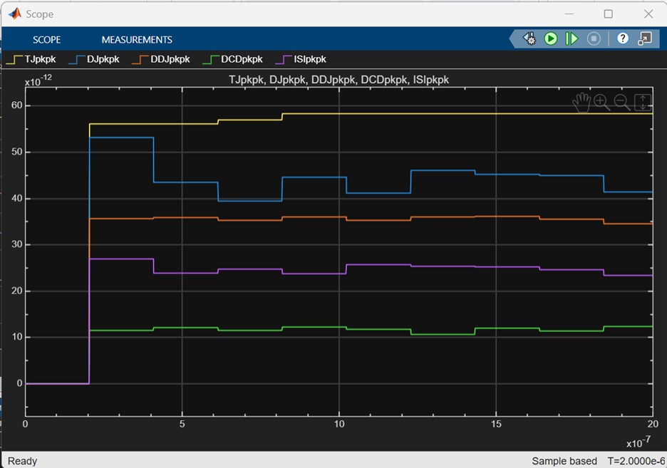
Figure 4: Jitter metrics update frame-by-frame for continuous visibility.

Improving ISI characterization in the system model

Similar to the waveform-based approach, because ISI-related jitter estimation depends on impulse response reconstruction, it can be more consistent to use a known channel impulse response and to set symbol levels accordingly.

This tends to stabilize ISI separation and can also reduce downstream distortion in other estimated components (notably RJ).

Getting Trustworthy Jitter Numbers: A Short Checklist

Whether you’re analyzing captured waveforms or measuring jitter inside a system-level SerDes simulation, a few practical checks go a long way:

• Validate thresholds and symbol time early: incorrect crossing detection ruins everything downstream.
• Use long enough frames (symbol decimation / number of UIs) to reduce estimate variance, especially for RJ and low-frequency periodic content.
• For sinusoidal jitter, remember the estimate uses FFT/DFT behavior: frequency-bin alignment matters, and phase is the most fragile.
• For ISI-related jitter, prefer supplying a known impulse response when possible; recovered impulse responses can pick up spurious behavior in the presence of other jitter sources.

Conclusion

Jitter isn’t just a pass/fail number, it’s a design feedback signal. When you can separate RJ vs DJ, identify periodic components, and quantify ISI-correlated timing shifts, you can make faster decisions about where to spend effort: clocking, equalization, channel modeling, or noise mitigation.

The two workflows above are complementary, so use the one that matches how you’re iterating your design.

• Use the waveform-based workflow when you want controlled impairment injection, component‑level validation, and sanity‑checking of measurement behavior.
• Use the in-model workflow when you want continuous visibility during long simulations, architectural iteration, or adaptive receiver convergence.

To try these workflows in detail, explore the step-by-step examples below.

• Model and Measure Jitter in Serial Data Systems

I’d love to hear your perspectives, please share your thoughts and experience in the comments below!

Interested to learn more? visit our MathWorks Solutions for Semiconductors Site