A previous post showed how to generate standalone C/C++ and CUDA source code directly from PyTorch and LiteRT models, with no runtime or inference engine, just portable source code compiled with your existing toolchain. That post started with a simple MLP to illustrate the idea. This one picks up where it left off and asks: what does this look like with a real model processing real video and deployed to real hardware?

The answer involves YOLOv26, a driving video, Simulink, and a Jetson AGX Orin. Let’s walk through it.

If you work in perception, including autonomous driving, robotics, industrial inspection, or video analytics, you’ve probably encountered YOLO at some point. YOLOv26 has a trick that makes it particularly appealing for code generation: no NMS. The model uses an end-to-end detection architecture with 300 learned object queries. Each query directly produces a unique detection: bounding box, confidence, class, and mask coefficients, without the non-maximum suppression step that traditionally complicates deployment.

This matters because NMS involves dynamic-length operations (sorting, filtering with unknown output size) that are less than ideal for static code generation. YOLOv26 sidesteps the problem entirely. You always get exactly 300 detections; just filter by confidence.

The updated model does instance segmentation: not just boxes, but pixel-level masks for each detected object.

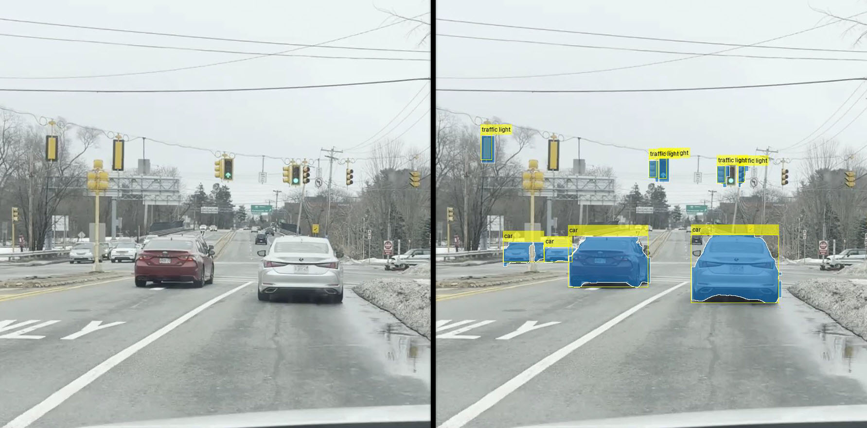
Detected vehicles and traffic lights from input video

We use the nano variant (~3M parameters, 6.7 MB). Small enough to run on edge hardware, accurate enough to be useful for our purposes.

Many state-of-the-art models are released as PyTorch checkpoints, and YOLOv26 is no exception. We start in Python to grab the pretrained model, wrap it to emit only the two outputs we need, and export to .pt2:

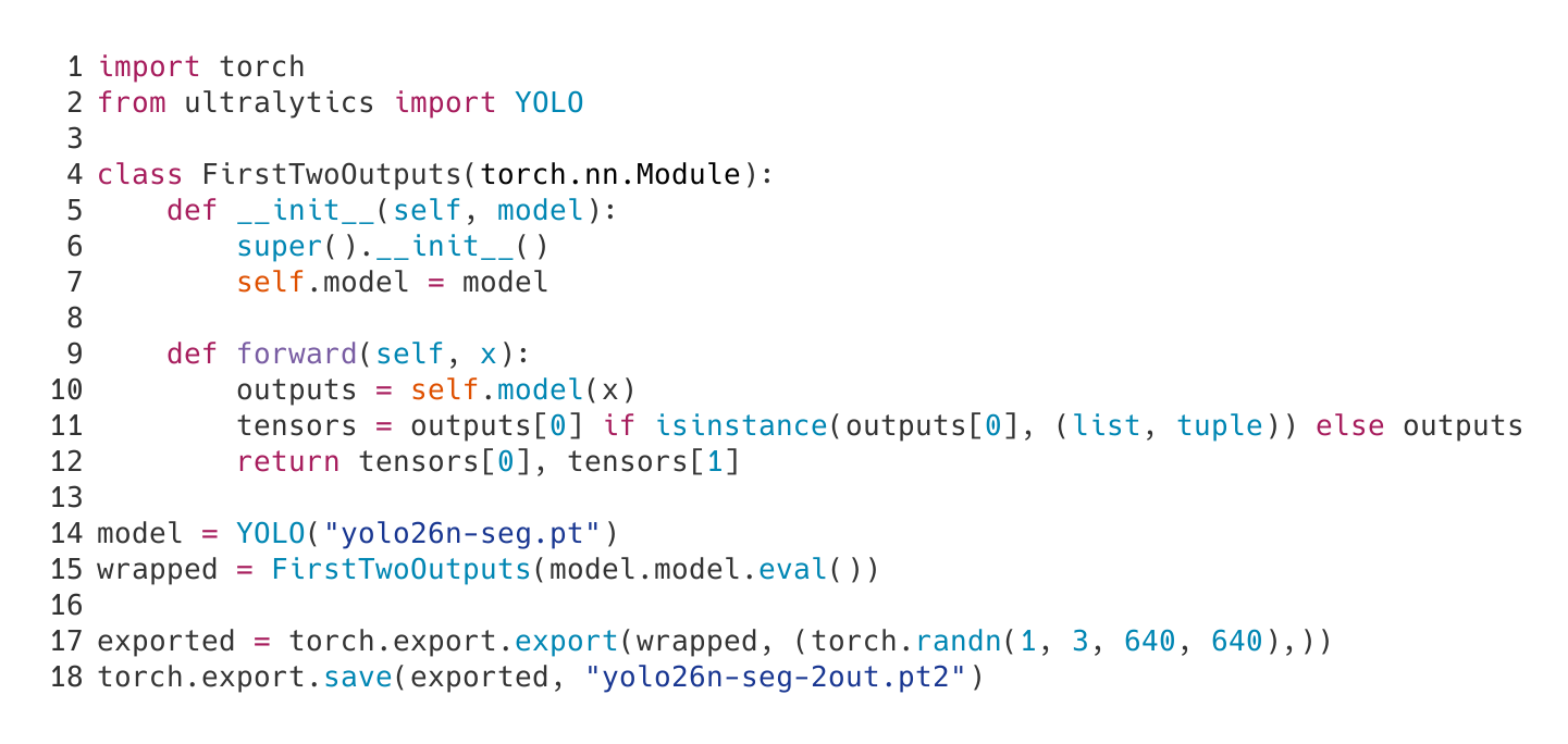
Python export wrapper for YOLOv26 nano

The .pt2 format (PyTorch ExportedProgram) freezes the computation graph into a static representation. No Python interpreter is needed at inference time and there is no dynamic dispatch, just the math that’s captured cleanly. This static representation is also what enables execution on edge devices. While the Jetson is a capable platform, every cycle counts when you run on the edge. When running your real-time application, you do not want the hardware to burn resources on a Python runtime and dynamic graph overhead alongside it.

We are not just checking that the file loads. We compare the exported model against the original PyTorch model on 128 COCO images, and the outputs match within floating-point tolerance. That gives us confidence that the next stages are validating deployment behavior, not debugging a PyTorch export mismatch.

Loading the model in MATLAB takes one line:

Load the PyTorch ExportedProgram in MATLAB

That loadPyTorchExportedProgram call from the MATLAB Coder Support Package for PyTorch and LiteRT Models is part of the entry-point function yoloSegmentImagePt2_v26.m, which wraps the full pipeline: resize, normalize, permute to PyTorch’s NCHW layout, run inference, filter by confidence, generate masks, and annotate. The permutation matches MATLAB image data to PyTorch’s tensor layout, ensuring YOLOv26 receives the input data in the expected shape and order. The function is designed from the start to be code generation-compatible:

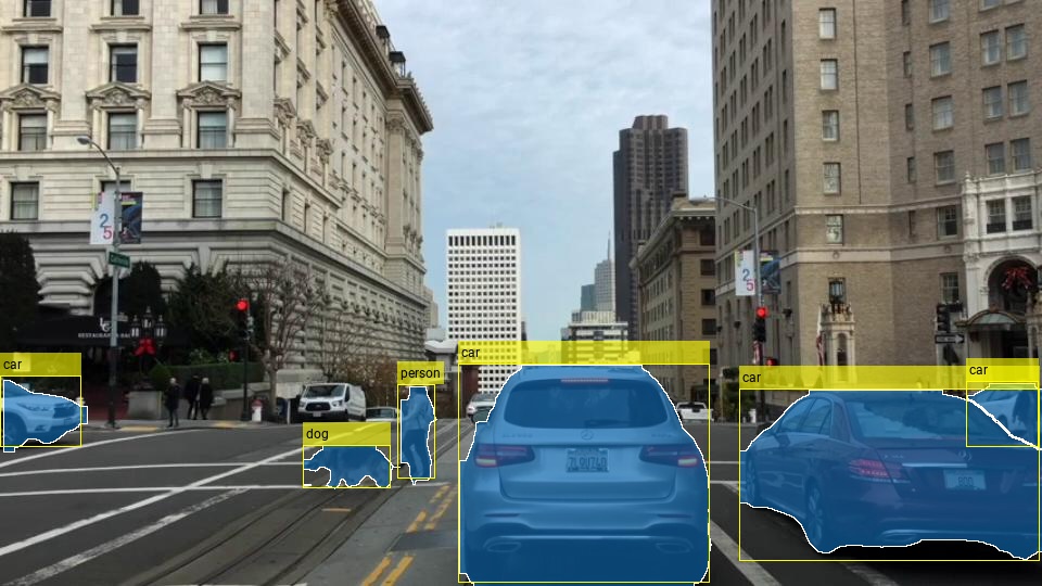
Run MATLAB inference on a test image

To verify we’re still getting the same results, we run the MATLAB interpretation against the full COCO128 dataset, the same 128 images used for Python validation. Detection counts and segmentation outputs match what we saw in Python, confirming that the .pt2 import preserves model behavior end-to-end.

But the whole point is to not stop at MATLAB interpretation. We want compiled code.

Generate C/C++ code with SIL verification

MATLAB Coder generates C/C++ source code, compiles it, and runs it on the host back-to-back with the MATLAB interpretation using Software-in-the-Loop (SIL) testing. The outputs match, verifying correctness on the x86 architecture before we move to any other target. We reuse the same testing infrastructure here to compare the generated code’s results against both MATLAB execution and the original Python outputs. Under the hood, the same MLIR-based optimizations from the previous post are at work: operator fusion, vectorization, and hardware-aware code emission.

Add coder.gpu.kernelfun to your entry-point function and replace coder.config with coder.gpuConfig in the build script to enable CUDA code generation using GPU Coder:

Generate CUDA code with SIL verification

The function and model don’t change, only the target language does. The generated CUDA kernels are standalone by default with no calls to cuDNN or TensorRT. Just CUDA code that compiles with nvcc (NVIDIA’s CUDA compiler) and runs on any modern NVIDIA GPU, whether that’s a desktop workstation, a Jetson, or a cloud instance with an A100.

If you do want to leverage TensorRT for optimized layer implementations and FP16 inference, simply replace with these two lines:

Optionally enable the generated CUDA to call TensorRT with FP16

The standalone path is simpler to deploy as it requires no library dependencies on the target while the TensorRT path trades that simplicity for runtime performance, though with an additional startup cost. Choose based on your constraints.

We used the MATLAB Agentic Toolkit with an AI coding agent throughout the Python and MATLAB sections. The agent acted on our behalf to call MATLAB and import the .pt2 file into the MATLAB code base, set up testing infrastructure, and iterate through the code generation steps for each target. This sped up development considerably, automating many of the steps needed to get our code up and running on the host machine.

With CUDA code generation working on the host, the next question is: does it run on the actual target hardware? GPU Coder will help us verify this by automating the deployment to the Jetson.

You don’t need to SSH into the Jetson and run commands manually. The entire deployment, including cross-compilation, file transfer, on-target builds, execution, and result retrieval, is orchestrated from MATLAB on your development machine. The jetson() hardware object gives you a programmatic connection to the device, and everything flows through it.

The deployment uses a two-phase build to handle a common cross-compilation wrinkle: we need OpenCV for image I/O on the Jetson, but it’s not installed on the Windows host. Linking at this stage would result in an error.

Phase 1 (from MATLAB on host): codegen cross-compiles the entry-point function into ARM64 .o files and transfers them to the Jetson automatically via the hardware object.

Phase 2 (triggered from MATLAB, runs on Jetson): MATLAB issues a system(hwobj, ...) call that compiles a custom C++/CUDA main on the Jetson, linking against the device’s local OpenCV and cuBLAS:

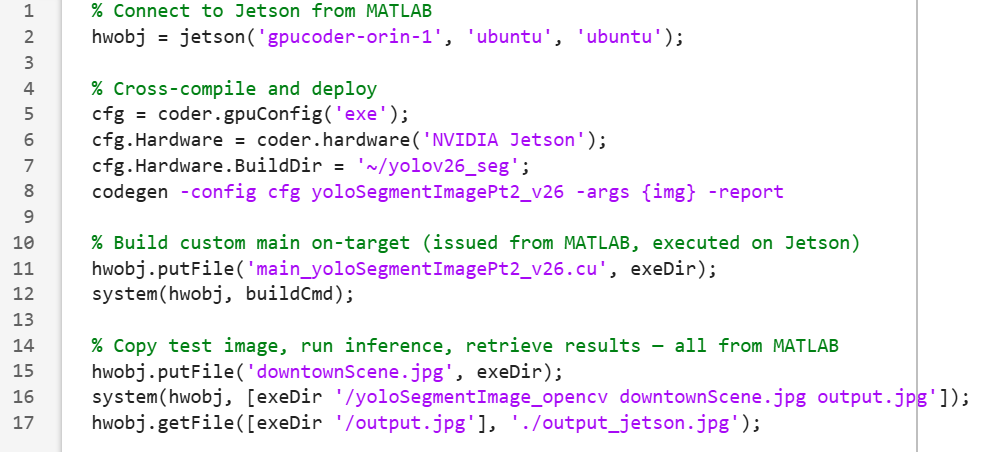
Deploy and run inference on Jetson from MATLAB

The custom main handles the layout conversion that every OpenCV-to-MATLAB bridge needs: BGR row-major (OpenCV) to RGB column-major (MATLAB-generated code) on input, and the reverse on output. It also includes a GPU warm-up step and inference timing.

Image processed on Jetson matches the results on host machine

The whole workflow (connect, cross-compile, transfer, build, run, retrieve) is wrapped in a single script (deployToJetson.m). One command from MATLAB, and you go from source code to running inference on the Jetson and viewing the result on your host.

With single-image inference validated on both host and Jetson, we move to video. If you’re building a perception system for a vehicle or a robot, you’re processing streams, frame after frame, in a pipeline that might include sensor fusion, control logic, and hardware I/O. That’s Simulink territory.

The YOLOv26Pt2VideoSimulink.slx model does exactly what you’d expect: reads a driving video (winter_driving.mp4), runs YOLOv26 on each frame, and overlays the segmentation results.

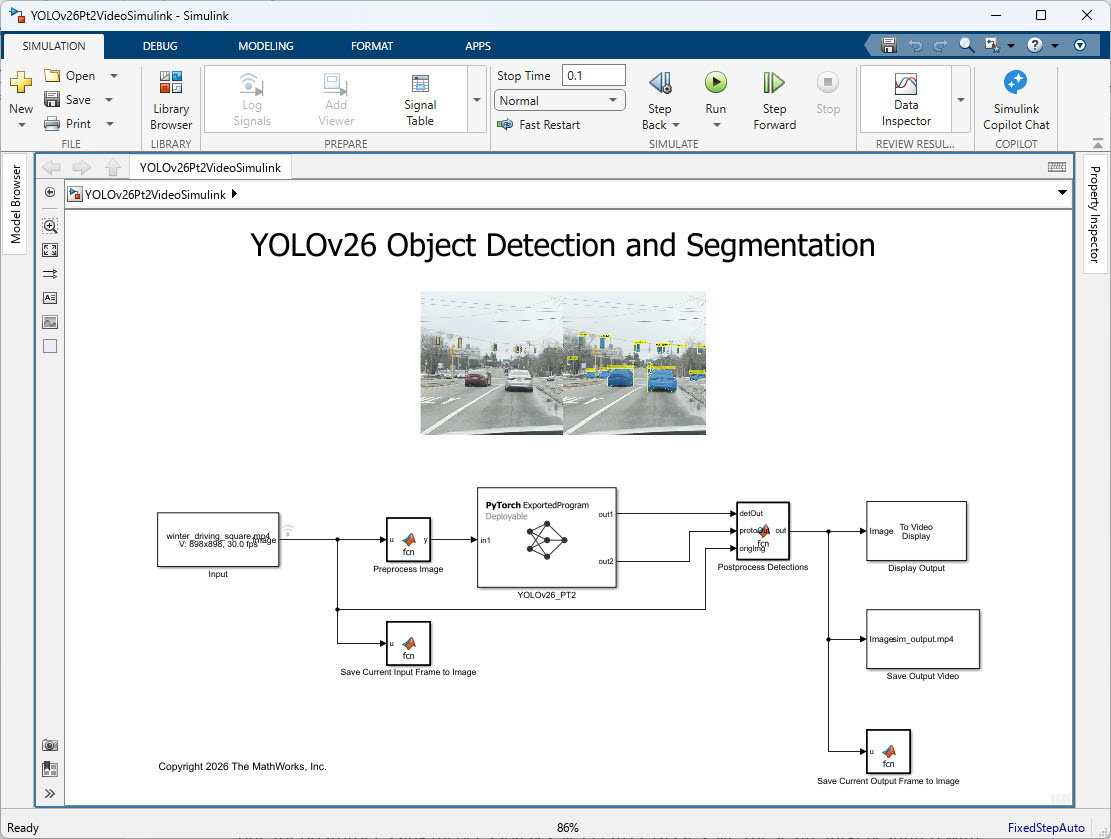
YOLOv26 in Simulink model processing input video

The interesting part is what’s inside: a PyTorch ExportedProgram block from the MATLAB Coder Support Package for PyTorch and LiteRT Models. This block loads the .pt2 file directly. You point it at the same yolo26n-seg-2out.pt2 file used previously in the MATLAB stage, configure the input/output dimensions, and it handles inference during simulation and generates C/C++/CUDA code when you build. Two MATLAB Function blocks flank it: one for preprocessing (resize, normalize), one for postprocessing (processMasks.m, createClasses.m). These are largely shared with the standalone MATLAB workflow, so little additional work was needed. The permutation to PyTorch’s NCHW layout? That’s handled inside the ExportedProgram block itself, so the flanking blocks stay simpler than in the standalone MATLAB path.

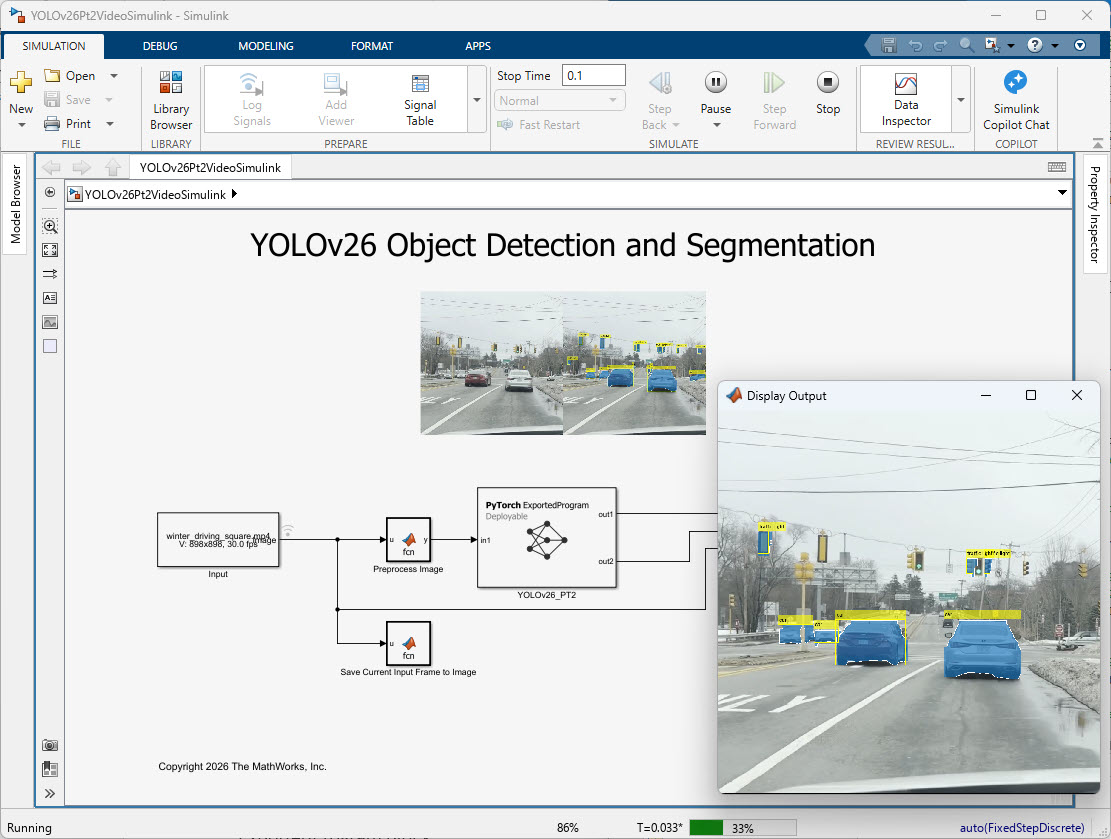
YOLOv26 running in Simulink with the detected objects in the output video stream

The output is an annotated video with colored segmentation masks, bounding boxes, and class labels for vehicles, pedestrians, and other road objects, all computed frame-by-frame inside Simulink.

We could have done all the Simulink work ourselves, but as we did with the MATLAB stage, we opted to use the Simulink Agentic Toolkit to help inspect block connections, verify signal dimensions, and iterate on the integration of the YOLOv26 network via the PyTorch ExportedProgram block.

Here’s what we’ve been building toward. We’ve validated the model in simulation. Now we generate CUDA code directly from the Simulink model:

Generating CUDA code from Simulink with GPU Coder

The %#codegen pragmas and coder.gpu.kernelfun calls in the helper functions tell GPU Coder to map parallelizable operations to CUDA kernels automatically. Since the pragmas and kernelfun calls were already in place from the MATLAB stage, we’re not doing anything extra here. We’re reusing the same code generation-ready functions. The PyTorch ExportedProgram block automatically generates optimized C/C++ or CUDA code to match the code generation settings configured in Simulink, so no additional configuration is needed. The result is standalone CUDA that processes the complete video pipeline: read frame, infer, post-process, annotate, and write frame.

Deploying to the Jetson is simpler this time around. We configure the same Jetson settings directly into the Simulink code generation settings, and Simulink + GPU Coder takes care of the rest. The end result is the same: cross-compiling the video pipeline for the Jetson’s ARM64 + CUDA architecture, managed from Simulink instead of the MATLAB command line.

A quick sidenote on how this workflow was developed. As briefly mentioned in previous sections, we paired the MATLAB Agentic Toolkit and Simulink Agentic Toolkit with an AI coding agent throughout this project. The toolkits give AI agents direct access to MATLAB and Simulink for running code, inspecting models, tweaking code generation settings, and diagnosing build failures.

This is especially valuable for the code generation steps, where users will often iterate as they tweak and tune the generated code running on the edge to match their requirements. Having an AI assistant that can run code generation, inspect the results, and retry shortens this loop considerably. And since the AI agents use MATLAB Coder and GPU Coder as trusted tools to generate C/C++ or CUDA code, you still get the same deterministic, reproducible output as if you were using those products directly. Finally, the toolkits are built on an open protocol (MCP) and so this approach extends to any AI assistant that supports it, including Codex, Gemini, or whatever comes next.

Here’s the pipeline in full:

The same YOLOv26 model and shared set of MATLAB functions carry you from interpreted prototyping through edge deployment, verified in Python, MATLAB, and Simulink environments along the way. The MATLAB Coder Support Package for PyTorch and LiteRT Models is what ties it together, bridging PyTorch’s research ecosystem with MATLAB and Simulink’s production deployment infrastructure.

If you’re working on perception for autonomous systems, robotics, or video analytics and want a traceable path from your PyTorch model to embedded hardware without hand-writing CUDA or managing inference runtimes, this is the workflow.