
Where am I? (The Localization Problem)
Autonomous Navigation with Brian Douglas: Part 4
This post is from Brian Douglas, YouTube content creator for Control Systems and Autonomous Applications.
In the previous post, I talked about the capabilities necessary for autonomous navigation. Over the next three posts, we’re going to explore one of those capabilities in more detail – localization. In this first post, we’re going to cover what localization is and what kind of information we need to accomplish it.
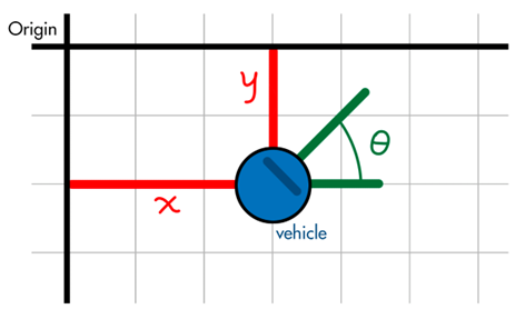
I want to start with a definition. A vehicle’s pose is the combination of its position and its orientation. It is where the vehicle is and which direction it’s facing. For example, if a vehicle can rotate about its vertical axis and move around on a flat 2D plane, then its pose can be described with a three-element vector. Its position on the 2D plane (the X and Y distance from some known reference frame), and its orientation (the angle theta off of the +X axis).
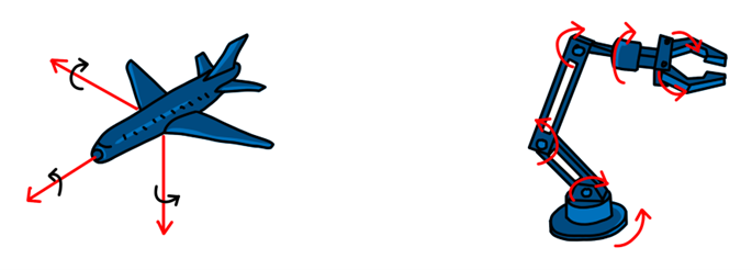
The number of elements needed to describe pose increases as the degrees of freedom (DOF) in the system increases. For example, an autonomous aircraft might require six elements to describe its pose: latitude, longitude and altitude for position, and roll, pitch, and yaw for its orientation. A robotic arm with multiple degrees of freedom could require many more elements than that.
Localization
Localization is the process of estimating the pose. It’s finding the value of each of the position and orientation elements such that the vehicle has an understanding of where it is and the direction it’s facing relative to the landmarks around it.
Simply put – if we give the vehicle a map of the environment, it should be able to figure out where it is inside that map.
Later in this blog series, we’re going to talk about how we can do localization when we don’t already have a map of the environment. This is the so-called Simultaneous Localization and Mapping (SLAM) problem. For now, we will assume the vehicle only needs to figure out where it is within a map that it already has.
So, what is a map?
A map is a model of the environment (Going forward, I’ll use map and model interchangeably when talking about how we represent the environment.), and the form that it takes depends on how we want to represent the world. With a map, we define the landmarks that are important to us and establish a coordinate system that we can use to quantify our relation to those landmarks.
Landmarks can be any number of physical things. For example, they could be the location of walls if the vehicle needs to navigate within a building. We could define a coordinate system that is referenced to one of the corners in the room and we could model the walls with a binary occupancy grid. This type of model divides the environment into a discrete number of smaller areas and then assigns a ‘1’ to areas that are occupied with a wall and ‘0’ to unoccupied areas.
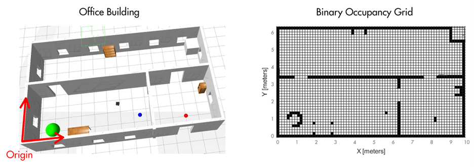
Localization would then consist of sensing the distance and direction to the walls of the environment and matching what you see to the binary occupancy grid to determine where you are.
However, a vehicle’s pose isn’t always described in relation to a landmark that is as easy to visualize as a wall. For example, we already said that a flying vehicle might describe its pose with latitude, longitude, altitude, roll, pitch, and yaw. These values describe the vehicle’s position in relation to geodetic coordinate system, and its orientation with a Local Vertical, Local Horizontal (LVLH) coordinate system. In this case, the map is quite simple as we only need to represent the shape of the Earth. We wouldn’t need the discrete details provided by a binary occupancy grid, and instead could model it as a continuous surface using a sphere, an oblate spheroid, a high order spherical harmonic model, or any other type of topographic map.
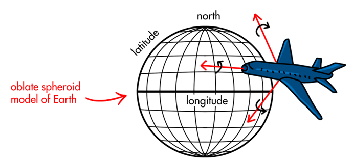
Localization for this vehicle could be done with GPS to find latitude, longitude, and altitude, and with an accelerometer to find down and a compass to find north.
To recap quickly, if the vehicle has a map of the environment, then localization is the process of sensing the environment and determining position and orientation within that map.
Example Scenario
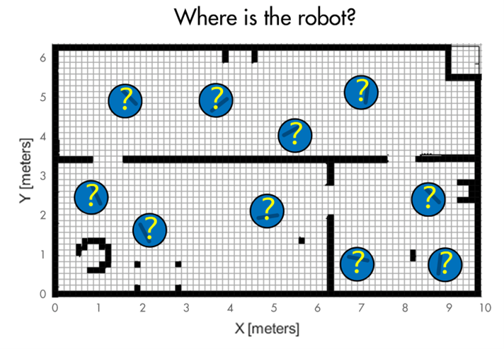
To understand this a bit better, let’s walk through a hypothetical localization problem. We have a robot that is wandering around an office building. The robot is given a map of the building in the form of a binary occupancy grid. Therefore, it knows the general layout of the walls and furniture but it doesn’t know initially where it is within the map – it could be anywhere. The problem is that the robot needs to use its sensors and motion models to estimate its pose, that is determine its position and orientation within the building.
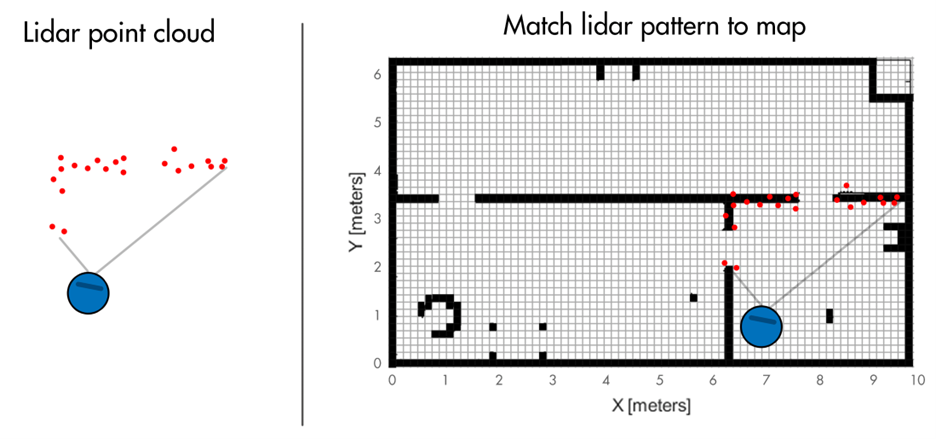
This robot has a Lidar sensor that returns the distance to objects within the field of view. So, if the sensor is looking at a corner and two doors, it might return a point cloud of dots that look like the drawing on the left. We can match this pattern to the map of the environment on the right and determine a possible robot location and orientation.
In addition to a noisy measurement, the robot also has a way to dead reckon its position using odometry data. Dead reckoning is when a future position is calculated using a past position and relative measurements like velocity and angular rate. For example, if you know the robot is facing north and moving at 1 meter per second, after 3 seconds you can estimate that the position is 3 meters north of where it used to be. You can have some confidence that the robot is there without having to observe the environment again.
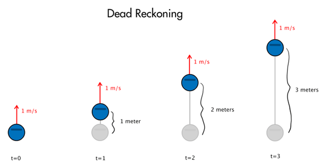
Dead reckoning can be used over shorter time frames with a lot of success but due to noise in the relative measurements, the error grows over time and needs to be corrected by measuring pose relative to the environment. For a more in depth understanding of dead reckoning, check out sensor fusion and tracking video number 3, where we combine the absolute measurement from a GPS with the relative measurement from an IMU.
We have two possible ways to determine location; we have a noisy lidar sensor that senses features that we can compare to a map of the environment and we have noisy odometry data that estimates how the robot is moving. If you are familiar with the Kalman filter, you might recognize that blending a noisy measurement with a noisy process model is exactly what it’s used for. If you’re not familiar with Kalman filters, you can get up to speed by watching this MATLAB tech talk series, but you shouldn’t need too much experience with them to understand the rest of this blog.
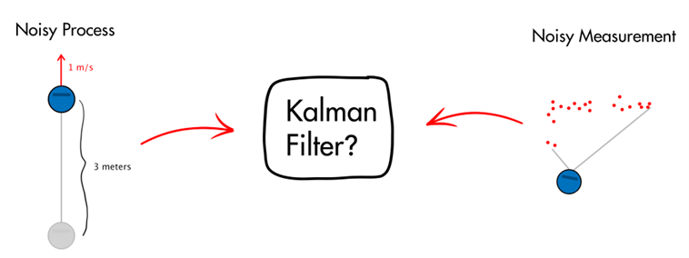
Unfortunately, a Kalman filter is not well suited for this localization problem. The main drawback is that it expects probability distributions to be Gaussian – or near Gaussian. For our problem, this means the random dead reckoning noise and the lidar measurement noise both need to be Gaussian. Which they might actually be, or at least close enough to still use a Kalman filter.
However, importantly the probability distribution of the estimated state of the robot must also be Gaussian, which we’ll see in the next blog post is definitely not the case for our localization example. Therefore, we need an estimation filter that can handle non Gaussian probability distributions. This is where the particle filter comes in.
To learn more on these capabilities, you can watch this detailed video on “Sensor Fusion and Navigation for Autonomous Systems using MATLAB and Simulink”. Thanks for sticking around till the end! If you haven’t yet, please Subscribe and follow this blog to keep getting the updates for the upcoming content. Also, we would love to hear from you about your robotics and autonomous systems projects in the comments section. Feel free to drop where you are with your journey!


评论
要发表评论,请点击 此处 登录到您的 MathWorks 帐户或创建一个新帐户。