
Object Creation Performance
Object Creation Performance
Back in January, we looked at the performance of creating a graphics object with a lot of data. Today we're going to look at what is basically the opposite problem. What does the performance look like when we're creating a lot of graphics objects which each have a tiny amount of data?
In general, creating a large number of graphics objects which each have a small amount of data is going to be slower than creating a small number of graphics objects with a large amount of data.
We can see this pretty easily with the following example. I want to draw a thousand markers along this curve:

t = linspace(0,2*pi,1000);
v = exp(i*t) - exp(6*i*t)/2 + i*exp(-14*i*t)/3;
x = real(v);
y = imag(v);
I could do this with 1,000 calls to scatter:
axes
hold on
s = 10;
drawnow
tic
for ix=1:1000
   scatter(x(ix),y(ix),s,t(ix),'filled');
end
drawnow
toc
Elapsed time is 7.610161 seconds.

Or I could do it with a single call to scatter:
hold off
cla
drawnow
tic
scatter(x,y,s,t,'filled')
drawnow
toc
Elapsed time is 0.056938 seconds.
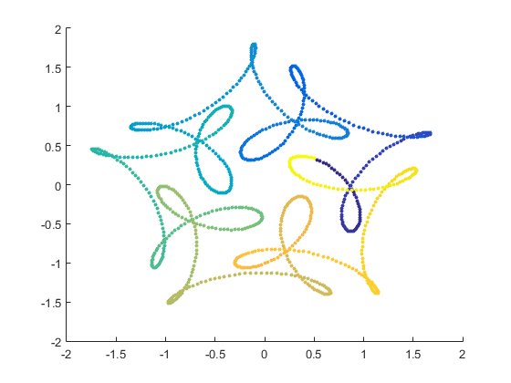
As you can see, creating a single scatter object with 1,000 points is about 150 times faster than creating 1,000 scatter objects which each have a single point.
But I want to generalize this and look at how it scales over different types and numbers of objects.
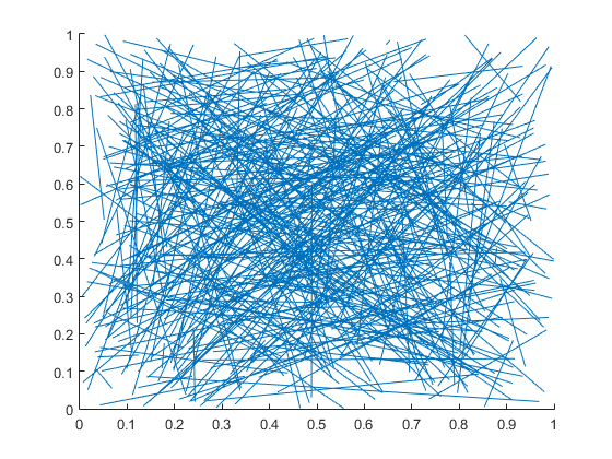
Lets start drilling into this by looking at the cost of creating 400 random lines. To get accurate data, I'll run this 15 times. That's because, as we'll see in a moment, there tends to be a bit of noise in these measurements. That's caused by other things running on the machine, where things are located in memory, and other things like that.
clf
drawnow
npass = 15;
results = zeros(1,npass);
x1 = rand(1,400);
x2 = rand(1,400);
y1 = rand(1,400);
y2 = rand(1,400);
for ix=1:npass
    cla
    drawnow
    tic
    for j=1:400
        line([x1(j) x2(j)],[y1(j) y2(j)])
    end
    drawnow
    results(ix) = toc;
end
I prefer to look at this type of data as 'Number of objects created per second', so we'll look at the number of objects divided by the time.
And we'll also want to look at the median of those 15 runs. The median is the best choice here because it's relatively insensitive to anomalies where one run "hiccups" because something else on the machine got resources.
grey = [.75 .75 .75];
plot(1:npass,400./results)
xlabel('Run #')
ylabel('Line objects per second')
min_lines_per_second = min(400./results);
median_lines_per_second = median(400./results)
max_lines_per_second = max(400./results);
line([1 15],repmat(min_lines_per_second,[1 2]),'Color',grey)
line([1 15],repmat(median_lines_per_second,[1 2]),'Color','green','LineWidth',2)
line([1 15],repmat(max_lines_per_second,[1 2]),'Color',grey)
ylim([0 inf])
median_lines_per_second =

   1.8366e+03
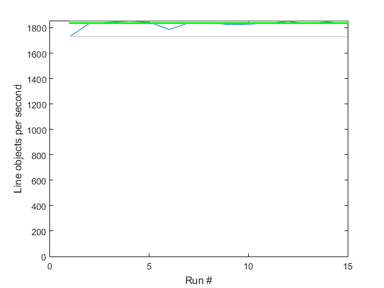
So the median is about 1,800 line objects per second.
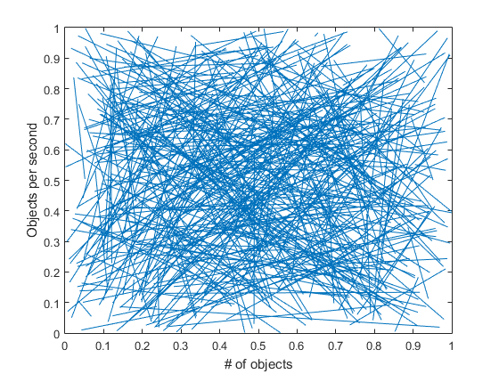
But as I said when we were looking at the large data case, it's always good to take a look at how performance scales with different size problems. I ran this same code, varying the number of objects from 0 to 500. I did 4 runs at each size and then saved the median values to a MAT file. You can see that there's still a bit of noise, but this is good enough to work with.
load R2015a_creation_results
plot(R2015a_creation_results.counts,R2015a_creation_results.counts./R2015a_creation_results.line_times);
hold on
errorbar(400,median_lines_per_second,median_lines_per_second-min_lines_per_second,max_lines_per_second-median_lines_per_second,'Color','red')
xlabel('# of objects')
ylabel('Objects per second')
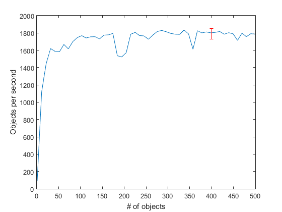
That looks pretty good. We can see that there's some startup cost, as we saw when scaling the amount of data, but we're pretty close to full speed once we get to about 150 objects.
Now that we've measured the performance of creating a graphics object, what can we do to speed it up when it's the bottleneck? The best thing we can do is obviously to create fewer objects, but how?
If you remember the post where I talked about performance scaling, then you may remember that the left side of the performance curves was flat. This means that the time it takes to create a line object with 2 points is pretty much the same as the time it takes to create a line object with 10,000 points. We can actually take advantange of that here by using a very old MATLAB graphics programming trick.
The basic idea is that you can put nan values into the X & Y data to break a line into multiple segments. To do this, we want to create arrays that look like this:
x3 = [x1(1), x2(1), nan, x1(2), x2(2), nan, x1(3), x2(3), nan, ...
y3 = [y1(1), y2(1), nan, y1(2), y2(2), nan, y1(3), y2(3), nan, ...
That's actually pretty easily done:
for ix=1:npass
    cla
    drawnow
    tic
    x3 = [x1; x2; nan(1,400)];
    y3 = [y1; y2; nan(1,400)];
    x3 = x3(:);
    y3 = y3(:);
    line(x3,y3)
    drawnow
    results(ix) = toc;
end
The performance of doing it this way is much, much better!
plot(1:npass,400./results)
xlabel('Run #')
ylabel('Line segments per second')
min_lines_per_second = min(400./results);
median_lines_per_second = median(400./results)
max_lines_per_second = max(400./results);
line([1 15],repmat(min_lines_per_second,[1 2]),'Color',grey)
line([1 15],repmat(median_lines_per_second,[1 2]),'Color','green','LineWidth',2)
line([1 15],repmat(max_lines_per_second,[1 2]),'Color',grey)
ylim([0 inf])
median_lines_per_second =

   3.5182e+04
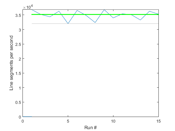
Well that certainly helped. We've gone from 1,800 lines per second up to 35,000 lines per second. That's almost a 20X speedup!
The problem with this old trick is that it isn't a one size fits all solution. You need to do things a little differently for different types of graphics objects. So we'll look at a couple of different types of graphics objects. While we do that, let's also look at the object creation performance in different versions of MATLAB.
Here's some data I collected for creating 7 different types of objects in each of the last 3 versions of MATLAB.
clf
load R2014a_create400_results
load R2014b_create400_results
load R2015a_create400_results
load R2015b_Prerelease_create400_results
plot_create400(R2014a_create400_results, ...
               R2014b_create400_results, ...
               R2015a_create400_results)
legend('R2014a','R2014b','R2015a')
title('Graphics Object Creation Performance')
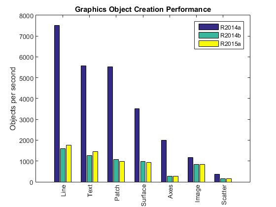
There's a lot going on in this chart. The first thing that we notice is that object creation took a big performance hit when the new graphics system was introduced in R2014b. That's because when the graphics objects got converted to real MATLAB classes, they lost a bunch of the performance tweaks that had been added to the old graphics system over the decades.
We can also see that the amount of slowdown depends on the type of object. It varies from taking taking about 40% longer to create an image, to taking about 7 times as long to create an axes. Both of those extremes are actually special cases. For most of the graphics objects (such as the line), the slowdown was about 4 times as long. We're slowly adding performance tweaks back into the new objects, as you can see for the line and text object in R2015a, but it will be quite a while before it catches up with the old system. This means that in any case where you need performance, you're going to want to optimize your code so you're not creating too many graphics objects. This was a good idea in earlier versions of MATLAB, but it is even more important in newer versions.
OK, so lets go back to our combining objects trick. The first thing to note is that it was already a good idea in older versions of MATLAB. That's why that trick of putting nans in to combine lines is an "old trick".
But how can we use the combining trick with these other objects?
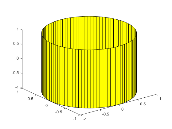
We've already seen how to combine calls to scatter and line. Patch is just a little bit trickier. If we're using the Face/Vertex form of patch, we can just concatenate the Vertices array, but we need to add an offset to one of the Faces arrays. So this:
clf
drawnow
tic
for ix=0:99
    a1 =  ix   *2*pi/100;
    a2 = (ix+1)*2*pi/100;
    v = [cos(a1), sin(a1), -1; ...
         cos(a2), sin(a2), -1; ...
         cos(a2), sin(a2),  1; ...
         cos(a1), sin(a1),  1];
    f = 1:4;
    patch('Vertices',v,'Faces',f,'FaceColor','yellow');
end
view(3)
drawnow
toc
Elapsed time is 0.111010 seconds.

Becomes this:
clf
drawnow
tic
verts = [];
faces = [];
for ix=0:99
    a1 =  ix   *2*pi/100;
    a2 = (ix+1)*2*pi/100;
    v = [cos(a1), sin(a1), -1; ...
         cos(a2), sin(a2), -1; ...
         cos(a2), sin(a2),  1; ...
         cos(a1), sin(a1),  1];
    f = 1:4;
    verts = [verts; v];
    faces = [faces; f + 4*ix];
end
patch('Vertices',verts,'Faces',faces,'FaceColor','yellow')
view(3)
drawnow
toc
Elapsed time is 0.026823 seconds.
Some of the others types of objects can be harder to combine though. The most important one is the axes. As we saw above, creating axes slowed down quite a bit in R2014b. That's largly because we've added a lot of features to the new version of axes. You've seen a couple of those features in the last two releases, but you'll be seeing a lot more of them when R2015b comes out this summer.
There are basically two different ways in which axes objects are used. The first is to actually use them as an axes to hold a chart. In this case, you want the ticks and labels and things. The other case is just as a container to draw something in. In this second case, you usually turn the Visible property of the axes off.
There isn't a lot you can do to combine axes in the first case. The subplot command will create a grid of axes, but it does that by actually creating a bunch of axes objects, so there isn't a shortcut there. The good news is that you usually don't create an awful lot of axes objects when you use them this way. Creating 400 axes objects in a single figure usually results in them being too small to read.
But in the second case, where we're turning the Visible property off, it often is pretty easy to combine several axes into a single object. Let's look at an example.
Here is an example from the MATLAB newsgroup.
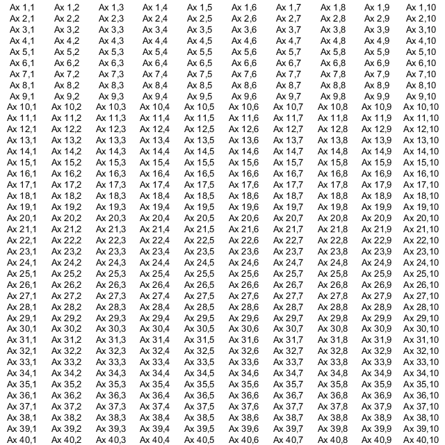
fw = 640;
fh = 640;
fig = figure('Units','pixels','Position',[0 0 fw fh]);
nRows = 40;
nKols = 10;
height = (fh-2)/nRows;
width = (fw-2)/nKols;
tic
for iRow = 1:nRows
    for iKol = 1:nKols
        axes('Units','pixels','Position',[1+(iKol-1)*width, fh-iRow*height, width, height], ...
             'Visible','off');
        text(.5,.5,['Ax ', num2str(iRow), ',', num2str(iKol)], ...
             'HorizontalAlignment','center')
    end
end
drawnow
toc
Elapsed time is 1.807279 seconds.
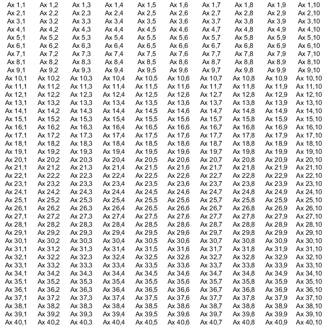
It's actually pretty easy to turn that into a single axes with a bunch of text objects in it:
delete(fig)
fig = figure('Units','pixels','Position',[0 0 fw fh]);
tic
axes('Position',[0 0 1 1],'Visible','off')
xlim([1 fw])
ylim([1 fh])
for iRow = 1:nRows
    for iKol = 1:nKols
        text(1+(iKol-.5)*width, fh-(iRow-.5)*height, ...
             ['Ax ', num2str(iRow), ',', num2str(iKol)], ...
             'HorizontalAlignment','center')
    end
end
drawnow
toc
Elapsed time is 0.567477 seconds.
That helps quite a bit, but we've still got all of those text objects. Unfortunately those are a lot harder to combine. We can combine all of the strings in one column by using a cell array:
delete(fig)
%clf
fig = figure('Units','pixels','Position',[0 0 fw fh]);
tic
axes('Position',[0 0 1 1],'Visible','off')
xlim([1 fw])
ylim([1 fh])
for iKol = 1:nKols
    strings = {};
    for iRow = 1:nRows
        strings{end+1} = ['Ax ', num2str(iRow), ',', num2str(iKol)];
    end
    text(1+(iKol-.5)*width, fw/2, strings, ...
             'HorizontalAlignment','center', ...
             'VerticalAlignment','middle');
end
drawnow
toc
Elapsed time is 0.175428 seconds.
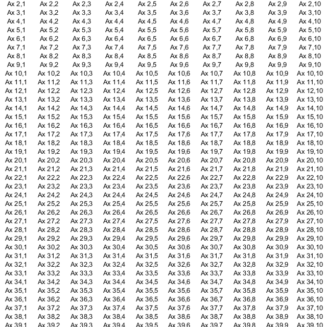
But as you can see, this isn't a perfect fix because it can be really hard to accurately control the vertical spacing. That means that you're only going to be able to use this approach for text in some special cases. You may find that the performance gain isn't enough to make up for the lose of placement control.
Both image and surface can also be tricky to combine into a single object. So the approach of combining several graphics objects into a single one isn't a perfect solution to the problem of object creation performance, but it is an important technique to know about when you're trying to make your MATLAB Graphics code run as fast as possible.
- カテゴリ:
- Performance

