FPLOT and Friends
Another new feature that I really like in R2016a is the upgraded fplot function and all of the new members of the fplot family.
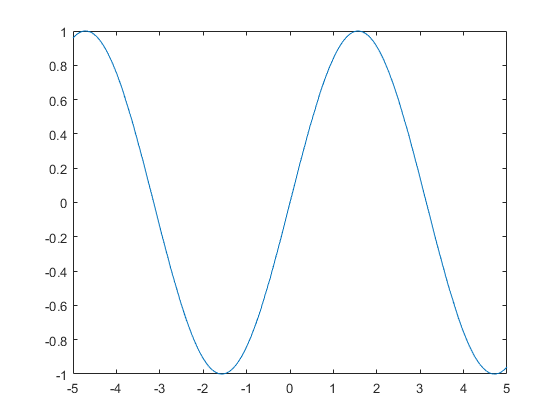
The fplot function has been around for a long time. The basic idea is that you pass it a function which takes X coordinates as inputs and returns Y coordinates as outputs. Then fplot will use that function to draw a curve.
fplot(@(x) sin(x))

This is really useful for getting a "quick feel" for the shape of a function, or a family of functions.
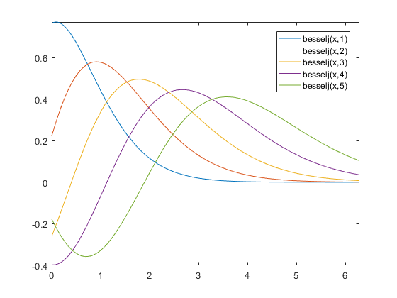
fplot(@(x) besselj(x,1),[0 2*pi])
hold on
fplot(@(x) besselj(x,2),[0 2*pi])
fplot(@(x) besselj(x,3),[0 2*pi])
fplot(@(x) besselj(x,4),[0 2*pi])
fplot(@(x) besselj(x,5),[0 2*pi])
hold off
legend show

In addition to functions, if you have the Symbolic Math Toolbox, fplot can also accept symbolic variables now. This gives it even more power. For example, I can reproduce that plot with a single call to fplot by calling besselj with a symbolic variable for the domain and a vector for the order.
syms x
fplot(besselj(x,1:5),[0,2*pi])
legend show

The new version of fplot has a lot of nice refinements, such as the nice legend entries in those last two examples.
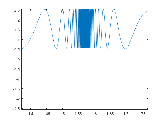
When we first showed the new fplot to Cleve, he gave it one of his favorite functions.
$$tan(sin(x)) + sin(tan(x))$$
This is what the previous version of fplot did with that.

And here's the R2016a version.
fplot(@(x) tan(sin(x)) + sin(tan(x)))

As you can see, it does a better of resolving the details in those tricky bits. And it labeled the asymptotes for use, although it missed the one at $-\pi/2$. The reason Cleve likes this function is that it's a bit of a torture test!
And we can get even more detail if we zoom in.
xlim(pi/2 + [-.2 .2])

Another big enhancement is that fplot can now do parametric curves as well as plotting Y as a function of X. To do this, we just pass it two functions. The first function takes the parameter value as input and returns X coordinates. The second function takes the parameter value as input and returns Y coordinates.
For example, I can use it to recreate the cubic Bézier curve from this blog post. This is a bit simpler than the way I did it in that post. Especially if you're not familiar with things like Kronecker tensor products. Note, you'll need the placelabel function I wrote in that earlier blog post.
clf
pt1 = [ 5;-10];
pt2 = [18; 18];
pt3 = [38; -5];
pt4 = [45; 15];
placelabel(pt1,'pt_1');
placelabel(pt2,'pt_2');
placelabel(pt3,'pt_3');
placelabel(pt4,'pt_4');
xlim([0 50])
axis equal
hold on

cubic_bezier = @(t,a,b,c,d) a*      (1-t).^3 ...
                        + 3*b*t   .*(1-t).^2 ...
                        + 3*c*t.^2.*(1-t)    ...
                        +   d*t.^3          ;

fplot(@(t)cubic_bezier(t,pt1(1),pt2(1),pt3(1),pt4(1)), ...
      @(t)cubic_bezier(t,pt1(2),pt2(2),pt3(2),pt4(2)), ...
      [0 1])

hold off

But one of the coolest features of the new version of fplot is hiding at the bottom of the doc page. If you look down there, you'll see this:
See Also
Functions
That's right, there's now a whole family of fplot-like functions!
Let's take a look at some of these new ones.
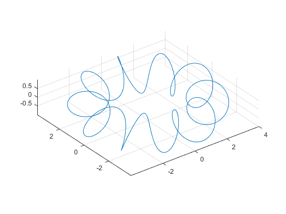
First there's fplot3. It's used for 3D parametric curves, like the ones I wrote about in these earlier posts on this blog (link1, link2). We just pass it 3 functions, like this:
fplot3(@(t) 3*cos(t)+cos(10*t).*cos(t), ...
       @(t) 3*sin(t)+cos(10*t).*sin(t), ...
       @(t) sin(10*t))
daspect([1 1 1])

Here's another of my favorite 3D parametric curves. It's commonly known as the baseball curve.
a = .4;
xfcn = @(t)sin(pi/2-(pi/2-a)*cos(t)).*cos(t/2+a*sin(2*t));
yfcn = @(t)sin(pi/2-(pi/2-a)*cos(t)).*sin(t/2+a*sin(2*t));
zfcn = @(t)cos(pi/2-(pi/2-a)*cos(t));

fplot3(xfcn,yfcn,zfcn,[0 4*pi])
axis equal

There's also the new fsurf function. This means that instead of calling peaks to generate arrays of data ...
[x,y,z] = peaks;
... and then passing that data to surf, ...
surf(x,y,z)
xlim([-3 3])
ylim([-3 3])
title('surf(peaks)')

I can just call fsurf with a handle to the peaks function.
fsurf(@(x,y) peaks(x,y),[-3 3 -3 3])
title('fsurf(@(x,y) peaks(x,y))')

This results in a very similar picture, but look what happens when we zoom in.

It's regenerating the mesh on the fly during the zoom. With the surf command, we'd only get the resolution of our original call to peaks.

This makes the fplot family really useful for exploring a function with pan and zoom.
All of the functions I've used so far have been simple enough to write as anonymous functions. But sometimes you'll want to use more complex functions. For example, I've turned the parametric equation for the Klein bottle into the following set of functions:
function x = klein_xfcn(u,v)
  mask1 = u<pi;
  mask2 = ~mask1;
  r = klein_rfcn(u);
  x = zeros(size(u));
  x(mask1) = 6*cos(u(mask1)).*(1+sin(u(mask1))) + r(mask1).*cos(u(mask1)).*cos(v(mask1));
  x(mask2) = 6*cos(u(mask2)).*(1+sin(u(mask2))) + r(mask2).*cos(v(mask2)+pi);
function y = klein_yfcn(u,v)
  mask1 = u<pi;
  mask2 = ~mask1;
  r = klein_rfcn(u);
  y = zeros(size(u));
  y(mask1) = 16*sin(u(mask1)) + r(mask1).*sin(u(mask1)).*cos(v(mask1));
  y(mask2) = 16*sin(u(mask2));
function z = klein_zfcn(u,v)
  r = klein_rfcn(u);
  z = r.*sin(v);
function r = klein_rfcn(u)
  r = 4*(1-cos(u)/2);
And now I can use fsurf to make a Klein bottle.
h = fsurf(@klein_xfcn,@klein_yfcn,@klein_zfcn,[0 2*pi 0 2*pi]);
camlight
axis equal
title('Klein Bottle')

And we can get a better idea of its shape by making it partially transparent.
h.EdgeColor = 'none';
h.FaceColor = [.929 .694 .125];
h.FaceAlpha = .5;
set(gca,'Projection','perspective')

There are a lot of goodies to play with in these functions, aren't there? And we haven't even talked about fmesh and fcontour.
- カテゴリ:
- Geometry


