
The Five Tetrahedra
The dodecahedron is a particularly interesting polyhedron. It's full of interesting five-fold symmetries. Let's take a look at a couple of them.
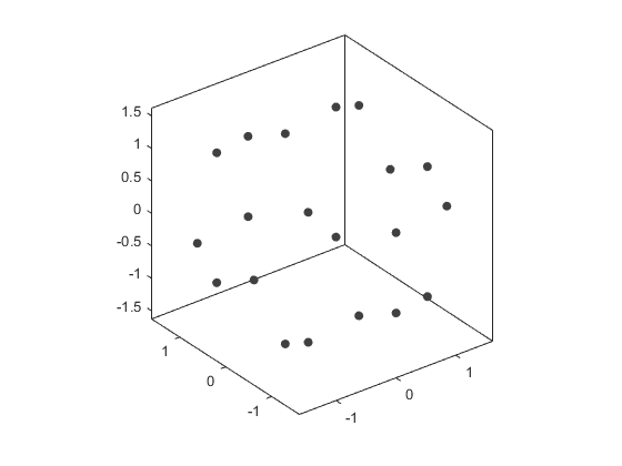
First we'll need the vertices. There's an interesting pattern to them.
p = (1+sqrt(5))/2;
q = 1/p;
verts = [-1 -1 -1; ...
         -1 -1  1; ...
          1 -1  1; ...
          1 -1 -1; ...
         -q  0 -p; ...
         -p -q  0; ...
          0 -p  q; ...
         -p  q  0; ...
          0 -p -q; ...
          q  0 -p; ...
         -q  0  p; ...
          0  p  q; ...
          p -q  0; ...
          0  p -q; ...
          p  q  0; ...
          q  0  p; ...
         -1  1  1; ...
         -1  1 -1; ...
          1  1 -1; ...
          1  1  1];
We can draw them with scatter3.
grey = [.25 .25 .25];
scatter3(verts(:,1),verts(:,2),verts(:,3),'filled','MarkerFaceColor',grey)
axis vis3d
grid off
box on
And we can draw the edges like so:
s = [1 1 1 2 2  2 3  3  3 4  4  4  5  5 6 7  8  8 10 11 11 12 12 12 13 14 14 15 15 16];
e = [5 6 9 6 7 11 7 13 16 9 10 13 10 18 8 9 17 18 19 16 17 14 17 20 15 18 19 19 20 20];
n = nan(1,30);
lx = [verts(s',1)'; verts(e',1)'; n];
ly = [verts(s',2)'; verts(e',2)'; n];
lz = [verts(s',3)'; verts(e',3)'; n];
l = line(lx(:),ly(:),lz(:),'Color',grey);

If you look at the first 4 vertices and the last 4 vertices, you might recognize that there's a cube hiding inside the dodecahedron. Let's draw it.
cols = lines(7);
faces = [ 4 19 20  3; ...
         19 18 17 20; ...
         18  1  2 17; ...
          1  4  3  2; ...
          2  3 20 17; ...
         18 19  4  1];
cube1 = patch('Faces',faces,'Vertices',verts,'FaceColor',cols(1,:));

Since everything in a dodecahedron comes in multiples of 5, lets make 4 more copies of that cube.
g2 = hgtransform;
cube2 = patch('Parent',g2,'Faces',faces,'Vertices',verts,'FaceColor',cols(2,:));
g3 = hgtransform;
cube3 = patch('Parent',g3,'Faces',faces,'Vertices',verts,'FaceColor',cols(3,:));
g4 = hgtransform;
cube4 = patch('Parent',g4,'Faces',faces,'Vertices',verts,'FaceColor',cols(4,:));
g5 = hgtransform;
cube5 = patch('Parent',g5,'Faces',faces,'Vertices',verts,'FaceColor',cols(5,:));
set([cube1 cube2 cube3 cube4 cube5],'SpecularStrength',0,'AmbientStrength',.4,'EdgeColor','none');

xlim([-p p])
ylim([-p p])
zlim([-p p])
camlight right

The cube has 4 diagonals which define axes of rotational symmetry. What if we start rotating each of those four extra cubes around one of those axes?
rotax = [1  1  1; ...
        -1  1 -1; ...
        -1 -1  1; ...
         1 -1 -1];
for ang=linspace(0,2*pi,250)
    g2.Matrix = makehgtform('axisrotate',rotax(1,:),ang);
    g3.Matrix = makehgtform('axisrotate',rotax(2,:),ang);
    g4.Matrix = makehgtform('axisrotate',rotax(3,:),ang);
    g5.Matrix = makehgtform('axisrotate',rotax(4,:),ang);
    drawnow
end

Something interesting happened at a particular angle in there. Did you see it? All of the vertices of the cubes land on vertices of the dodecahedron. It happens when the angle reaches pi/4.
ang = pi/4;
g2.Matrix = makehgtform('axisrotate',rotax(1,:),ang);
g3.Matrix = makehgtform('axisrotate',rotax(2,:),ang);
g4.Matrix = makehgtform('axisrotate',rotax(3,:),ang);
g5.Matrix = makehgtform('axisrotate',rotax(4,:),ang);

It can be a little easier to see some of the symmetry patterns if we make all of the cubes the same color and add some different edges.
set(findobj(gca,'Type','patch'),'FaceColor',cols(5,:))
s = [1  1  1  1  2  2  2  2  2  3  3  3  3  3  4  4  4  5  5  5  5  6  6  6  6  6  7 ...
     7  7  8  8  8  9 10 10 10 10 11 11 12 12 12 12 13 13 13 14 14 14 15 16 17 17 18 19];
e = [2  7  8 18  3  8  9 16 17  4  9 11 15 20  7 15 19  6  8 14 19  7  9 11 17 18 11 ...
    13 16 11 12 14 13 13 14 15 18 12 20 15 16 18 19 16 19 20 15 17 20 16 17 18 20 19 20];
n = nan(1,55);
lx2 = [verts(s',1)'; verts(e',1)'; n];
ly2 = [verts(s',2)'; verts(e',2)'; n];
lz2 = [verts(s',3)'; verts(e',3)'; n];
l.XData = lx2(:);
l.YData = ly2(:);
l.ZData = lz2(:);
l.LineWidth = 3;

There are also tetrahedra hiding inside the dodecahedron. Let's draw one of them.
delete(findobj(gca,'Type','patch'))
l.XData = lx(:);
l.YData = ly(:);
l.ZData = lz(:);
l.LineWidth = .5;

faces = [2  5 12; ...
         2  5 13; ...
         2 12 13; ...
         5 12 13];
tet1 = patch('Faces',faces,'Vertices',verts);
tet1.FaceColor = cols(1,:);

Again, we'll make 5 copies of this.
g2 = hgtransform;
tet2 = patch('Parent',g2,'Faces',faces,'Vertices',verts,'FaceColor',cols(2,:));
g3 = hgtransform;
tet3 = patch('Parent',g3,'Faces',faces,'Vertices',verts,'FaceColor',cols(3,:));
g4 = hgtransform;
tet4 = patch('Parent',g4,'Faces',faces,'Vertices',verts,'FaceColor',cols(4,:));
g5 = hgtransform;
tet5 = patch('Parent',g5,'Faces',faces,'Vertices',verts,'FaceColor',cols(5,:));
set([tet1 tet2 tet3 tet4 tet5],'SpecularStrength',0,'AmbientStrength',.4,'EdgeColor','none');

And we'll spin these around four different axes. In this case, the axes of rotation are each through the midpoint of an edge which touches one of the vertices of the tetrahedron.
r = 1+p;
rotax = [-1, -r,  p; ...
         -p,  1, -r; ...
         -1,  r,  p; ...
          r, -p, -1];

for ang=linspace(0,2*pi,250)
    g2.Matrix = makehgtform('axisrotate',rotax(1,:),ang);
    g3.Matrix = makehgtform('axisrotate',rotax(2,:),ang);
    g4.Matrix = makehgtform('axisrotate',rotax(3,:),ang);
    g5.Matrix = makehgtform('axisrotate',rotax(4,:),ang);
    drawnow
end

This one's a bit harder to follow, but there is one particularly interesting angle in this case too. When the angle of rotation reaches pi, all of the vertices of the tetrahedra land on vertices of the dodecahedron.
ang = pi;
g2.Matrix = makehgtform('axisrotate',rotax(1,:),ang);
g3.Matrix = makehgtform('axisrotate',rotax(2,:),ang);
g4.Matrix = makehgtform('axisrotate',rotax(3,:),ang);
g5.Matrix = makehgtform('axisrotate',rotax(4,:),ang);
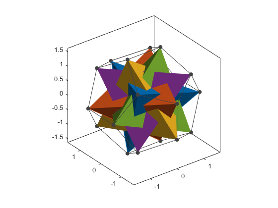
The pattern can be a little hard to see at first, but if we look straight down on one of the faces of the dodecahedron, it jumps out at us.
view(0,60)

If we combine the tetrahedra, we get an interesting shape that was first described by Edmund Hess in 1876, who also described that compound of the five cubes.
set(findobj(gca,'Type','patch'),'FaceColor',cols(5,:))
axis off
delete(findobj(gca,'Type','line'))
delete(findobj(gca,'Type','scatter'))

One of the unusual features of this shape is that it is an enantiomorph of its dual. Enantiomorphs are shapes which are mirror images of each other. There's another object which is a mirror image of this one. Coxeter called this one the "dextro" version. Here's the other one, which is known as the "laevo" version.
first_ax = gca;
first_ax.Position = [.05 .05 .4 .8];
title(first_ax,'Dextro')
second_ax = copyobj(first_ax,first_ax.Parent);
second_ax.Position = [.55 .05 .4 .8];
delete(findobj(second_ax,'Type','patch'))

faces = [8  9 19; 8 16  9; 8 19 16;  9 16 19; ...
         5  7 15; 5 17  7; 5 15 17;  7 17 15; ...
         3  6 12; 3 10  6; 3 12 10;  6 10 12; ...
         1 11 13; 1 14 11; 1 13 14; 11 14 13; ...
         2  4 18; 2 20  4; 2 18 20;  4 20 18];
hlaevo = patch('Faces',faces,'Vertices',verts, ...
               'FaceColor',cols(5,:),'EdgeColor','none', ...
               'SpecularStrength',0,'AmbientStrength',.4, ...
               'Parent',second_ax);
title(second_ax,'Laevo')

The dextro and laevo versions look similar, but you can't rotate one of them in such a way as to make it match the other one.
If we combine a dextro and a laevo in the same axes, we get another interesting object, but that's a story for another day.
hlaevo.Parent = first_ax;
delete(second_ax)
first_ax.Position = [0 0 1 1];
title(first_ax,'')

I've always found these 5-way symmetries fascinating. What do you think?
- Category:
- Geometry

