Linear Programming, the HiGHS Optimization library and MATLAB
What is linear programming?
Linear programming (LP) is a mathematical method used to determine the best possible outcome (such as maximum profit or lowest cost) in a mathematical model whose requirements are represented by linear relationships. It involves optimizing a linear objective function, subject to a set of linear constraints (equalities and inequalities).
Put more formally, we want to find the vector x that minimizes the function
subject to the constraints
whereAand are matrices while f, b, , lb and ub are vectors.
For me, this makes more sense when looking at a specific example.So, let's consider the classic diet problem as described in [1]. Suppose you have three foods available: Corn, Milk and Bread
Food | Cost / Serving | Vitamin A | Calories | Maximum servings |
Corn (C) | $0.18 | 107 | 72 | 10 |
Milk (M) | $0.23 | 500 | 121 | 10 |
Bread (B) | $0.05 | 0 | 65 | 10 |
You also have two nutritional requirements to satisfy
Nutrient | Minimum amount in diet | Maximum amount in diet |
Calories | 2,000 | 2,250 |
Vitamin A | 5,000 | 50,000 |
and you can have a maximum of 10 portions of any one food type.
How would you choose the foods that minimise the cost while satisfying all of the constraints?
In MATLAB, here's how to solve this using the Problem-based approach, which is the easiest way to get started with solving linear programs in MATLAB. An alternative method would be to use the solver-based approach, which we'll look at later.
% How many servings of each food to eat each day
C = optimvar("corn", LowerBound = 0,UpperBound = 10);
M = optimvar("milk", LowerBound = 0,UpperBound = 10);
B = optimvar("bread",LowerBound = 0,UpperBound = 10);
prob = optimproblem;
prob.Objective = C*0.18 + M*0.23 + B*0.05; % The cost to minimise
% Add constraints for the Vitamin A requirements
prob.Constraints.c1 = C*107 + M*500 >= 5000;
prob.Constraints.c2 = C*107 + M*500 <= 50000;
% Add constraints for the Calories requirements
prob.Constraints.c3 = C*72 + M*121 + B*65 >= 2000;
prob.Constraints.c4 = C*72 + M*121 + B*65 <= 2250;
diet = solve(prob)
The solve function tells us that it decided to use the linprog function to find the solution, useful information if we ever decide to switch to the-solver based approach in the future.
The result tells us that the cheapest solution is to have 10 portions of bread, 1.944 portions of corn and 10 portions of milk. To see how much this costs, we evaluate the objective function at the solution point.
cost = evaluate(prob.Objective, diet);
fprintf("The optimal diet would cost $%.2f\n",cost)
This is a very small problem with only 3 variables; you may even be able to solve it by hand!
Real linear problems are difficult to solve
Real problems tend to be much larger with many thousands of variables and constraints. In addition, there is a class of linear programs called Mixed Integer Linear Programs (MILP) which have the extra constraint that some or all entries of the solution vector be integers.
Solving them can be very difficult! Indeed, there is a collection called MIPLIB 2017 (to which MathWorks is a contributor) that contains problems so hard that even the best solvers in the world can't tackle them. To get your head around this, consider that an easy problem in the MIPLIB 2017 collection is defined as something that can be solved in less than an hour on a machine with 16 cores. That's a lot of compute for something that's defined as 'easy'.
Let's take a look at one such 'easy' problem from MIPLIB 2017 using the latest version of MATLAB, R2024b. The problem is called acc-tight5 and is a basketball scheduling instance that's stored in the MPS file format.
% Download and unzip the MPS file containing the problem
gunzip("https://miplib.zib.de/WebData/instances/acc-tight5.mps.gz")
problem = mpsread("acc-tight5.mps")
The mpsread function creates a structure that is suitable for the solver-based approach to solving linear programs and also tells us which solver we should use: intlinprog, since this is a mixed integer problem.
acc_tight5_solution = intlinprog(problem);
We can see that intlinprog took 84.4 seconds to solve this problem and that, like the mpsread function, it uses something called HiGHS. We switched to using the HiGHS library by default in MATLAB R2024a for both linprog and intlinprog, while mpsread started using it in R2024b. You can get a clue as to why we switched to HiGHS by asking intlinprog to use its original solver, the one that was used by default until recently.
options = optimoptions("intlinprog",Algorithm="legacy");
problem.options = options;
acc_tight5_solution_old = intlinprog(problem);
At 1617.9 seconds, the legacy algorithm took rather longer, 20x longer in fact. Now such amazing speed-ups won't always be the case. Sometimes, HiGHS is only a little faster, other times it can even be slower. When considering many problems the transition was worth making.
What is HiGHS?
HiGHS is high performance software for solving large-scale sparse linear programming (LP), mixed-integer programming (MIP) and quadratic programming (QP) models. It is developed in C++11, with interfaces to several other languages.The name HiGHS comes from the initials of its original developers.
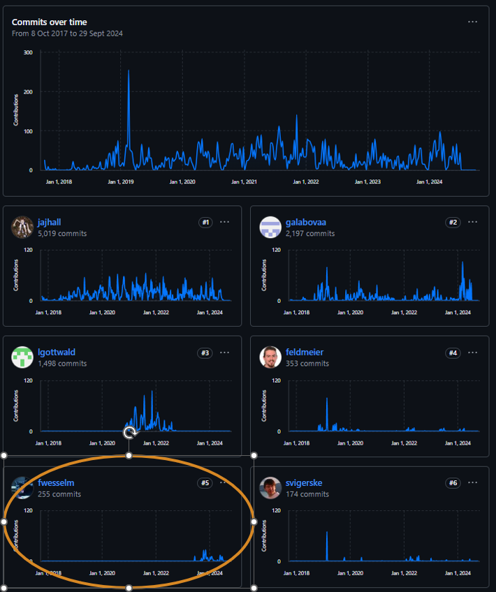
Back in June 2024 I had the pleasure of attending the first ever HiGHS workshop at The University of Edinburgh of which MathWorks was one of the sponsors and where MathWorks developer, Franz Wesselmann, was one of the speakers. While there I met Julian Hall and Ivet Galabova who are responsible for three of the initials in HiGHS and are the current maintainers and leaders of the project. MathWorks has been working closely with them for a while now as we worked towards incorporating HiGHS into MATLAB via Optimization Toolbox.

One of the contributions that MathWorks makes back into the HiGHS project is to work directly on the code. MathWorker Franz Wesselmann is now in the top 5 contibutors to the project in terms of numbers of commits.
This is a fruitful collaboration for all concerned and you can expect more HiGHS-related functionality coming to MATLAB in the future. Thanks to everyone in the HiGHS team for welcoming us to their community.
References
[1] The Diet Problem: A WWW-based Interactive Case Study in Linear Programming. Joseph Czyzyk and Timothy J. Wisniewski


コメント
コメントを残すには、ここ をクリックして MathWorks アカウントにサインインするか新しい MathWorks アカウントを作成します。