
Generating Hilbert curves
This week I came across some files I wrote about 16 years ago to compute Hilbert curves. A Hilbert curve is a type of fractal curve; here is a sample:
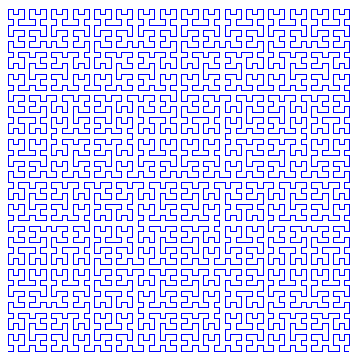
I can't remember why I was working on this. Possibly I was anticipating that 16 years in the future, during an unusually mild New England winter, I would be looking for a blog topic.
Anyway, there are several interesting ways to code up a Hilbert curve generator. My old code for generating the Hilbert curve followed the J. G. Griffiths, "Table-driven Algorithms for Generating Space-Filling Curves," Computer-Aided Design, v.17, pp. 37-41, 1985. Here's the basic procedure:
First, initialize four curves, \( A_0 \), \( B_0 \), \( C_0 \), and \( D_0 \), to be empty (no points).
Then, build up the Hilbert curve iteratively as follows:
\[ A_{n+1} = [B_n, N, A_n, E, A_n, S, C_n] \]
\[ B_{n+1} = [A_n, E, B_n, N, B_n, W, D_n] \]
\[ C_{n+1} = [D_n, W, C_n, S, C_n, E, A_n] \]
\[ D_{n+1} = [C_n, S, D_n, W, D_n, N, B_n] \]
where \( N \) represents a unit step up, \( E \) is a unit step to the right, \( S \), is a unit step down, and \( W \) is a unit step left.
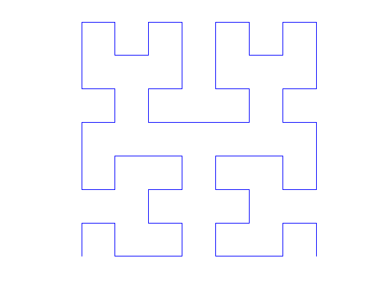
One way to code this procedure is to incrementally build up a set of vectors that define the step from one point on the path to the next, and then to use a cumulative summation at the end to turn the steps into x-y coordinates. Here's how you might do it.
A = zeros(0,2);
B = zeros(0,2);
C = zeros(0,2);
D = zeros(0,2);

north = [ 0  1];
east  = [ 1  0];
south = [ 0 -1];
west  = [-1  0];

order = 3;
for n = 1:order
  AA = [B ; north ; A ; east  ; A ; south ; C];
  BB = [A ; east  ; B ; north ; B ; west  ; D];
  CC = [D ; west  ; C ; south ; C ; east  ; A];
  DD = [C ; south ; D ; west  ; D ; north ; B];

  A = AA;
  B = BB;
  C = CC;
  D = DD;
end

A = [0 0; cumsum(A)];

plot(A(:,1), A(:,2), 'clipping', 'off')
axis equal, axis off
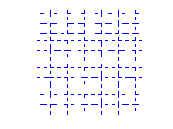
I was curious to see what might be on the MATLAB Central File Exchange, so I searched for "hilbert curve" and found several interesting contributions. There are a couple of 3-D Hilbert curve generators, and several different ways of coding up a 2-D Hilbert curve generator. I was particularly interested in the Fractal Curves contribution by Jonas Lundgren.
Jonas shows a much more compact implementation of the ideas above using complex arithmetic. It looks like this:
a = 1 + 1i;
b = 1 - 1i;

% Generate point sequence
z = 0;
order = 5;
for k = 1:order
    w = 1i*conj(z);
    z = [w-a; z-b; z+a; b-w]/2;
end

plot(z, 'clipping', 'off')
axis equal, axis off
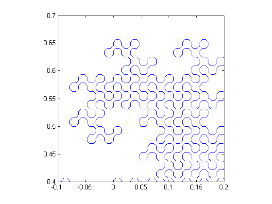
Jonas' contribution includes several other curve generators. Here's one called "dragon".
z = dragon(12);
plot(z), axis equal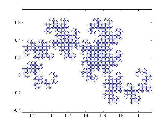
Here's a zoom-in view of a portion of the dragon.
axis([-.1 0.2 0.4 0.7])
What do you think? Does anyone know of an image processing application for shape-filling curves? Please leave a comment.


See Also
-

The Dragon Curve
Blogs
-
Interactive Curve Class
Blogs


コメント
コメントを残すには、ここ をクリックして MathWorks アカウントにサインインするか新しい MathWorks アカウントを作成します。