
Revised Circularity Measurement in regionprops (R2023a)
For some shapes, especially ones with a small number of pixels, a commonly-used method for computing circularity often results in a value which is biased high, and which can be greater than 1. In releases prior to R2023a, the function regionprops used this common method. In R2023a, the computation method has been modified to correct for the bias.
For the full story, read on!
What Is Circularity?
Our definition of circularity is:
$c = \frac{4\pi a}{p^2}$
where a is the area of a shape and p is its perimeter. It is a unitless quantity that lies in the range $[0,1]$. A true circle has a circularity of 1. Here are the estimated circularity measurements for some simple shapes.
url = "https://blogs.mathworks.com/steve/files/simple-shapes.png";
A = imread(url);
p = regionprops("table",A,["Circularity" "Centroid"])
imshow(A)
for k = 1:height(p)
text(p.Centroid(k,1),p.Centroid(k,2),string(p.Circularity(k)),...
Color = "yellow",...
BackgroundColor = "blue",...
HorizontalAlignment = "center",...
VerticalAlignment = "middle",...
FontSize = 14)
end
title("Circularity measurements for some simple shapes")

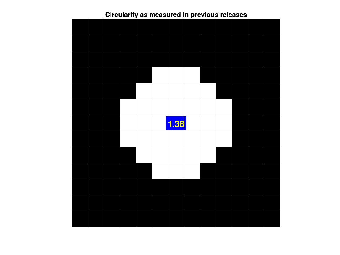
Circularity > 1??
Some users have been understandably puzzled to find that, in previous releases, regionprops sometimes returned values greater than 1 for circularity. For example:
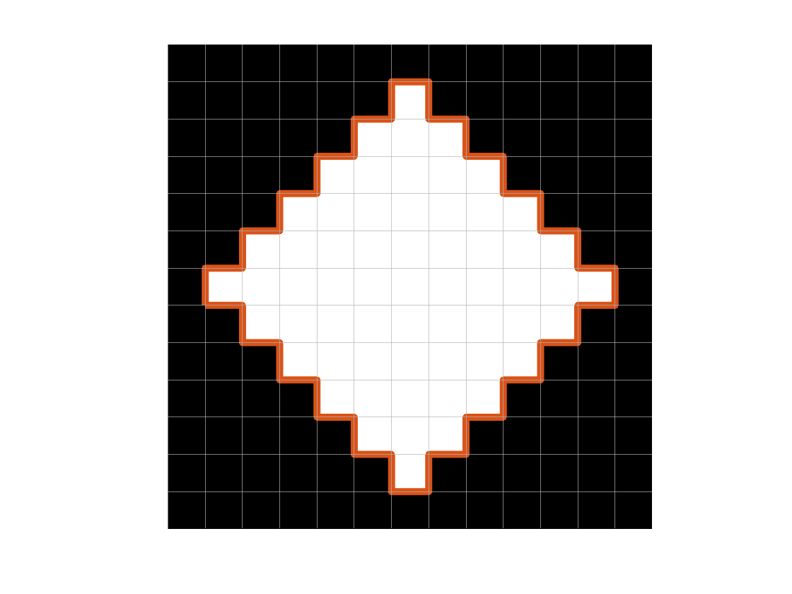
url = "https://blogs.mathworks.com/steve/files/small-circle.png";
B = imread(url);
imshow(B)
outlinePixels(size(B))
text(7,7,"1.38",...
Color = "yellow",...
BackgroundColor = "blue",...
HorizontalAlignment = "center",...
VerticalAlignment = "middle",...
FontSize = 14)
title("Circularity as measured in previous releases")
Measuring Perimeter
Before going on, I want to pause to note that, while circularity can be a useful measurement, it can also be quite tricky. One can get lost in fractal land when trying to measure perimeter precisely; see Bernard Mandelbrot's famous paper, "How Long Is the Coast of Britain? Statistical Self-Similarity and Fractional Dimension," described on Wikipedia here. Then, add the difficulties introduced by the fact that we are working with digital images, whose pixels we sometimes think of as points on a discrete grid, and sometimes as squares with unit area. See, for example, MATLAB Answers MVP John D'Errico's commentary on this topic.
In fact, measuring perimeter is what gets the common circularity computation method in trouble. Measuring the perimeter of objects in digital images is usually done by tracing along from one pixel center to the next, and then adding up weights that are determined by the angles between successive segments.
b = bwboundaries(B);
imshow(B)
outlinePixels(size(B))
hold on
plot(b{1}(:,1),b{1}(:,2),Color = [0.850 0.325 0.098],...
Marker = "*")
hold off
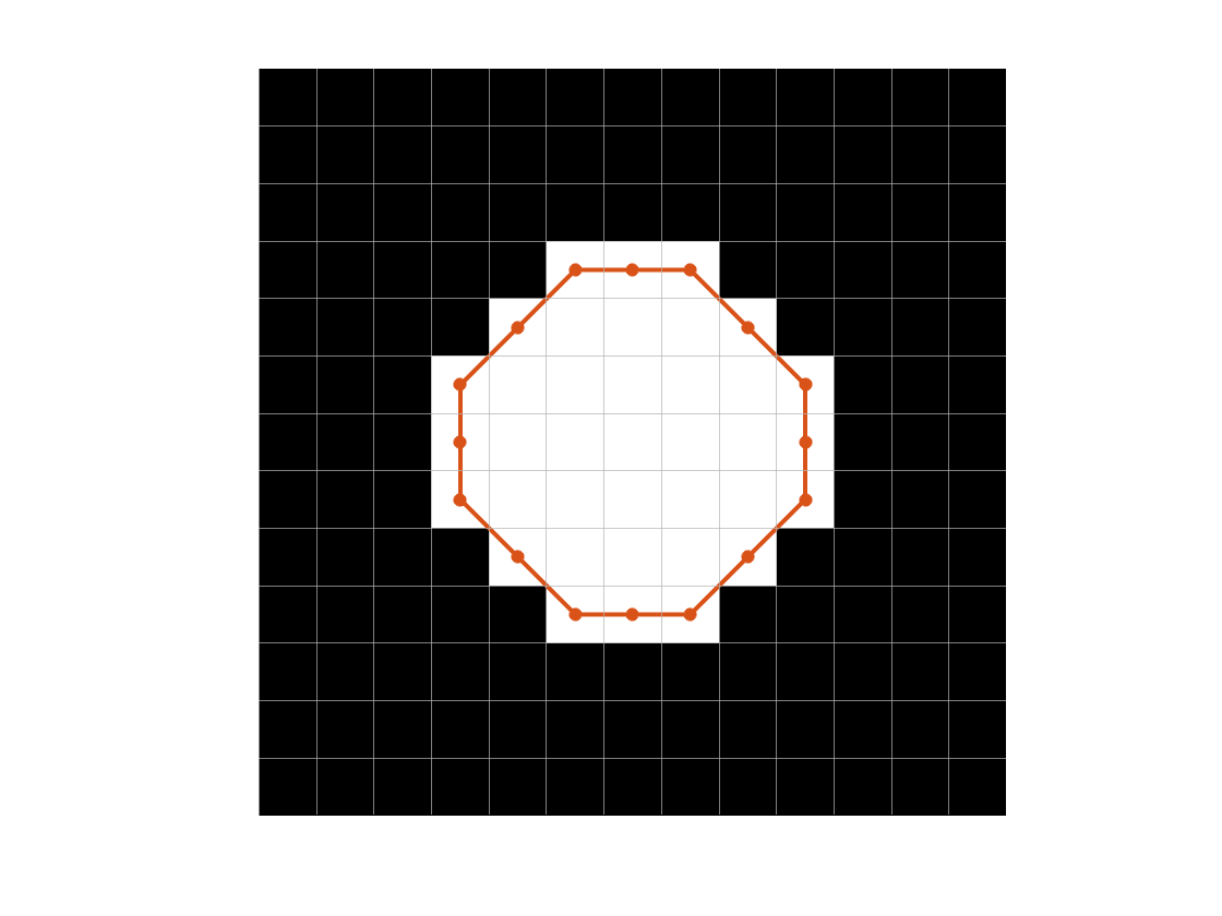
A few different schemes have been used to assign the weights in order to minimize systematic bias in the perimeter measurement. The weights used by regionprops are those given in Vossepeol and Smeulders, "Vector Code Probability and Metrication Error in the Representation of Straight Lines of Finite Length," Computer Graphics and Image Processing, vol. 20, pp. 347-364, 1982. See the discussion in Luego, "Measuring boundary length," Cris' Image Analysis Blog: Theory, Methods, Algorithms, Applications, https://www.crisluengo.net/archives/310/, last accessed 20-Mar-2023.
The cause of the circularity computation bias can be seen in the figure above. The perimeter is being calculated based on a path that connects pixel centers. Some of the pixels, though, lie partially outside the red curve. The perimeter, then, is being calculated along a curve that does not completely contain all of the square pixels; the curve is just a bit too small. Relative to the area computation, then, the perimeter computation is being underestimated. Since perimeter is in the denominator of the circularity formula, the resulting value is too high.
Can we fix the problem by tracing the perimeter path differently? Let's try with a digitized square at a 45-degree angle.
mask = [ ...
0 0 0 0 0 0 0 0 0 0 0 0 0
0 0 0 0 0 0 1 0 0 0 0 0 0
0 0 0 0 0 1 1 1 0 0 0 0 0
0 0 0 0 1 1 1 1 1 0 0 0 0
0 0 0 1 1 1 1 1 1 1 0 0 0
0 0 1 1 1 1 1 1 1 1 1 0 0
0 1 1 1 1 1 1 1 1 1 1 1 0
0 0 1 1 1 1 1 1 1 1 1 0 0
0 0 0 1 1 1 1 1 1 1 0 0 0
0 0 0 0 1 1 1 1 1 0 0 0 0
0 0 0 0 0 1 1 1 0 0 0 0 0
0 0 0 0 0 0 1 0 0 0 0 0 0
0 0 0 0 0 0 0 0 0 0 0 0 0 ];
Here is the path traced by regionprops for computing the perimeter.
x = [1 6 11 6 1] + 1;
y = [6 1 6 11 6] + 1;
imshow(mask)
outlinePixels(size(mask))
hold on
plot(x,y,Color = [0.850 0.325 0.098])
hold off
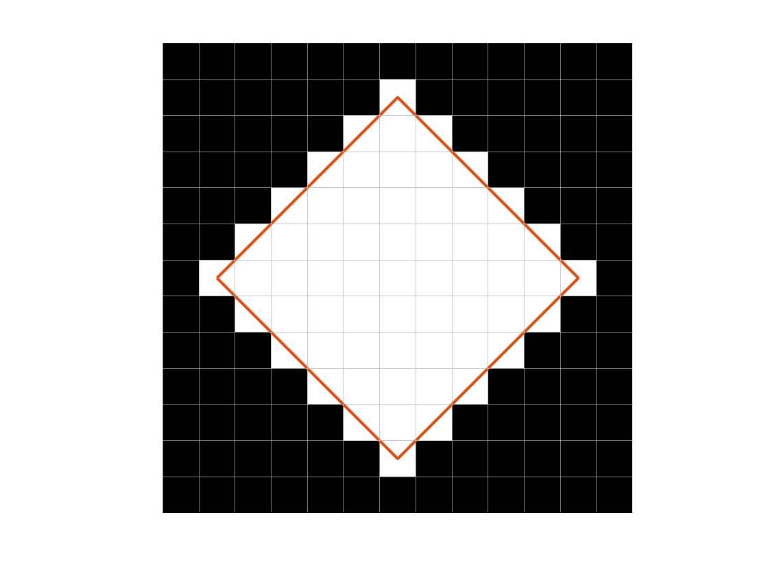
The perimeter of the red square is $4 \cdot 5 \sqrt{2} \approx 28.3$. The would correspond to an area of $(5 \sqrt{2})^2$. However, the number of white squares is 61. The estimated perimeter and area are inconsistent with each other, which will result in a biased circularity measurement.
Can we fix it by tracing the perimeter along the outer points of the pixels, like this?
x = [1.5 6.5 7.5 12.5 12.5 7.5 6.5 1.5 1.5];
y = [6.5 1.5 1.5 6.5 7.5 12.5 12.5 7.5 6.5];
imshow(mask)
outlinePixels(size(mask))
hold on
plot(x,y,Color = [0.850 0.325 0.098])
hold off
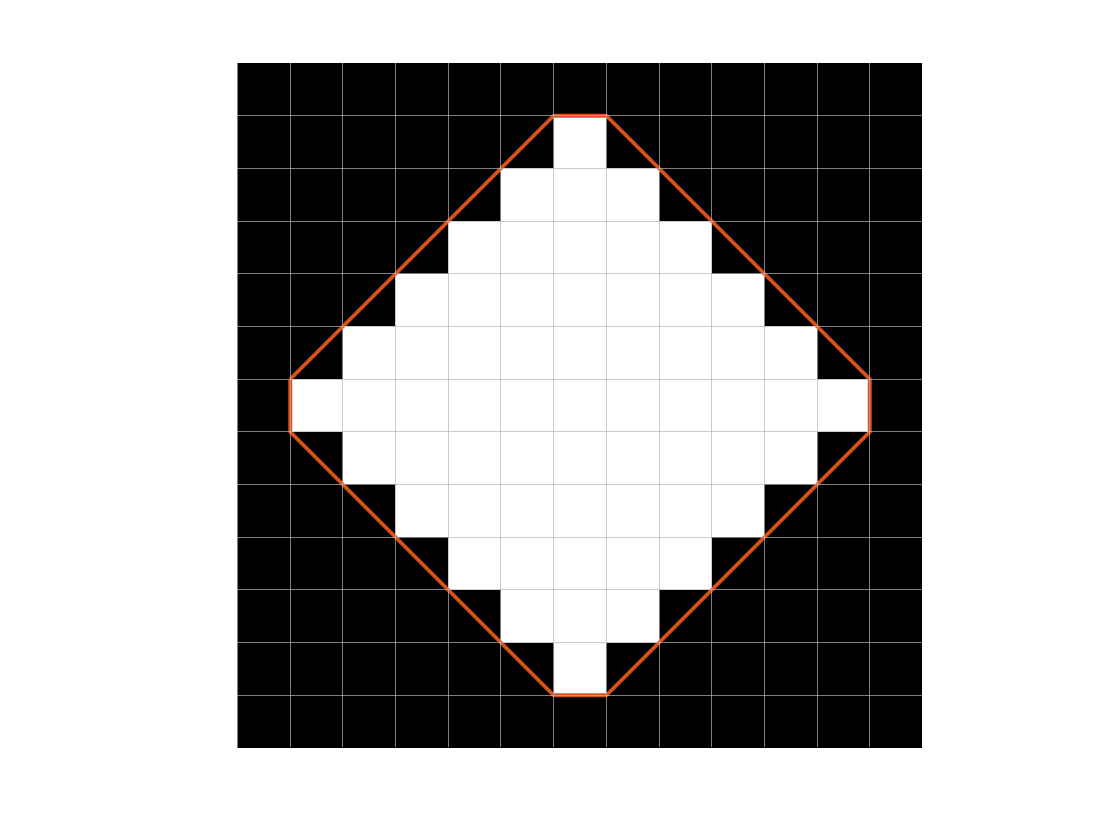
Now the calculated perimeter is going to be too high because it corresponds to an area that is much greater than 61, the number of white pixels.
perim = sum(sqrt(sum(diff([x(:) y(:)]).^2,2)))
For a square, that perimeter corresponds to this area:
area = (perim/4)^2
This time, the estimated perimeter is too high with respect to the estimated area, and so the computed circularity will be biased low.
What if we compute the perimeter by tracing along the pixel edges?
x = [1.5 2.5 2.5 3.5 3.5 4.5 4.5 5.5 5.5 6.5 6.5 ...
7.5 7.5 8.5 8.5 9.5 9.5 10.5 10.5 11.5 11.5 12.5 12.5 ...
11.5 11.5 10.5 10.5 9.5 9.5 8.5 8.5 7.5 7.5 6.5 6.5 ...
5.5 5.5 4.5 4.5 3.5 3.5 2.5 2.5 1.5 1.5];
y = [7.5 7.5 8.5 8.5 9.5 9.5 10.5 10.5 11.5 11.5 ...
12.5 12.5 11.5 11.5 10.5 10.5 9.5 9.5 8.5 8.5 ...
7.5 7.5 6.5 6.5 5.5 5.5 4.5 4.5 3.5 3.5 2.5 2.5 1.5 1.5 ...
2.5 2.5 3.5 3.5 4.5 4.5 5.5 5.5 6.5 6.5 7.5];
imshow(mask)
outlinePixels(size(mask))
hold on
plot(x,y,Color = [0.850 0.325 0.098], LineWidth = 5)
hold off
But now the calculated perimeter is WAY too high with respect to the area, so the computed circularity would be very low.
perim = sum(sqrt(sum(diff([x(:) y(:)]).^2,2)))
Bias Correction Model
After all that, we decided to leave the perimeter tracing method alone. Instead, we came up with a simple approximate model for the circularity bias and then used that model to derive a correction factor.
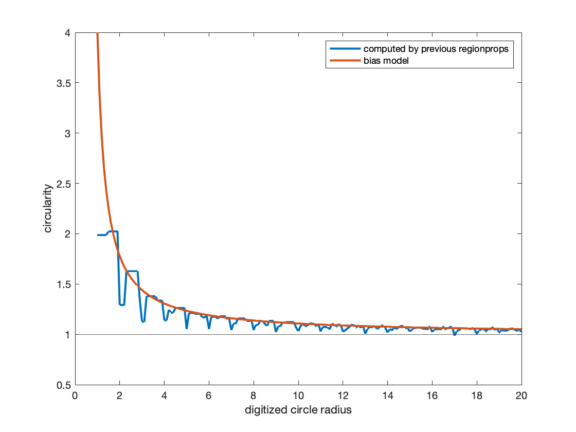
Consider a circle with radius r. We can model the bias by computing circularity using area that is calculated from r and perimeter that is calculated from $r - 1/2$. The result, $c'$, is the model of the biased circularity.
$c' = \frac{1}{1 - \frac{1}{r} + \frac{0.25}{r^2}} = \frac{1}{\left(1 - \frac{0.5}{r}\right)^2}$
How well does $c'$ match what the old regionprops computation was returning? Here is a comparison performed on digitized circles with a range of radii.
But what should we do for general shapes? After all, if we already know it's a circle, then there's no big need to compute the circularity metric, right?
Here's the strategy: Given the computed area, a, determine an equivalent radius, $r_{\text{eq}}$, which is the radius of a circle with the same area. Then, use $r_{\text{eq}}$ to derive a bias correction factor:
$c_{\text{corrected}} = c\left(1 - \frac{0.5}{r_{\text{eq}}}\right)^2 = c\left(1-\frac{0.5}{\sqrt{a/\pi}}\right)^2$
Does It Work?
We just made a big assumption there, computing $r_{\text{eq}}$ as if our shape is a circle. Can we really do that? Well, we did a bunch of experiments, using various kinds of shapes, scaled over a large range of sizes, and rotated at various angles. Here are the results for one experiment, using an equilateral triangle with a base rotated off the horizontal axis by 20 degrees. The blue curve is the circularity computed in previous releases; the red curve is the corrected circularity as computed in R2023a, and the horizontal orange line is the theoretical value.

We saw similar curves for a broad range of shapes. For some shapes, with a theoretical circularity value below around 0.2, the correction did not improve the result. On balance, however, we decided that the correction method was worthwhile and that regionprops should be changed to incorporate it.
If you need to get the previously computed value in your code, see the Version History section of the regionprops reference page for instructions.
Helper Function
function outlinePixels(sz)
M = sz(1);
N = sz(2);
for k = 1.5:(N-0.5)
xline(k, Color = [.7 .7 .7]);
end
for k = 1.5:(M-0.5)
yline(k, Color = [.7 .7 .7]);
end
end


Comments
To leave a comment, please click here to sign in to your MathWorks Account or create a new one.