
Sinusoids and FFT frequency bins
Contents
Note: I really didn't expect to be writing about the FFT two weeks in a row. But ready or not, here we go!
My friend Joe walked into my office the other day and announced, "Steve, I've got a question about the FFT."
(Joe was one of my MathWorks interviewers 21 years ago this month. His question for me then was, "So what do you bring to the party?" I don't remember how I answered.)
Joe is one of the biggest MATLAB experimenters I know. He's always trying to use MATLAB for some new kind of analysis or to automate something dubious (such as changing the hue of the lights in his house. Hmm.)
Anyway, lately he's been into automatic analysis of music. And something was bothering him. If you have a pure sinusoid signal and take the FFT of it, why does it spread out in the frequency domain? How do you interpret the output of fft when the frequency is in between two adjacent frequency bins of the FFT? And is that situation fundamentally different somehow that when the sinusoid's frequency is exactly one of the FFT bin frequencies?
Oh boy. I told Joe, "Well, you don't really have a sinusoid. A sinusoid is an infinitely long signal. You have a finite portion of a sinusoid, which I think of as a rectangularly windowed sinusoid. Go away, let me think more about how to explain all that, and then I'll come find you tomorrow."
Because of my background in digital signal processing, I tend to think about this in terms of the relationships between three kinds of Fourier transforms:
- Fourier transform (continuous time - continuous frequency)
- discrete-time Fourier transform (DTFT) (discrete time - continuous frequency
- discrete Fourier transform (DFT) (discrete time - discrete frequency)
I have written before (23-Nov-2009) about the various kinds of Fourier transforms. It is this last kind, the DFT, that is computed by the MATLAB fft function.
It's hard to tell exactly where to start in any discussion about Fourier transform properties because the use of terminology and the mathematical convensions vary so widely. Let me just dive in and walk through Joe's example. If you have questions about what's going on, please post a comment.
Note: In what follows, I am making a very big simplifying assumption. Specifically, I'm assuming that the sampling frequency is high enough for us to be able to discount the possibility of aliasing in the sampling of the sinusoid. This isn't a completely valid assumption because, unlike a real sinusoid, the truncated or windowed sinusoid doesn't have a finite bandwidth.
Here some sample parameters that Joe gave me.
Sinusoid frequency in Hz:
f0 = 307;
Sampling frequency in Hz:
Fs = 44100;
Sampling time:
Ts = 1/Fs;
How many samples of the sinusoid do we have? From a theoretical perspective, think of this as the length of a rectangular window that multiplies our infinitely long sinusoid sequence.
M = 1500;
Construct the signal
n = 0:(M-1);
y = cos(2*pi*f0*Ts*n);
Compute M-point discrete Fourier transform (DFT) of f. This is what the function fft computes.
Y = fft(y);
Plot the DFT. The DFT itself doesn't have physical frequency units associated with it, but we can plot it on a Hz frequency scale by incorporating our knowledge of the sampling rate. (I'm plotting the DFT as disconnected points to emphasize its discrete-frequency nature. Also, I'll be plotting magnitudes of the Fourier transforms throughout.)
f = (0:(M-1))*Fs/M;
plot(f,abs(Y),'*')
xlim([0 Fs/2])
title('Magnitude of DFT')
xlabel('Frequency (Hz)')

Exploring the "spread" around the peak
Zoom in on the peak.
p = 2*Fs/(M+1);
f1 = f0 - 10*p;
f2 = f0 + 10*p;
xlim([f1 f2])

What's with the "spread" around the peak? The spread is caused by the fact that we do not have a pure sinusoid. We have only a finite portion of a pure sinusoid.
To explore this further, let's relate the DFT to what some might call the "real" Fourier transform of our windowed sinusoid. If we can discount aliasing, then the discrete-time Fourier transform (DTFT) is the same as the "real" Fourier transform up to half the sampling frequency. And, for a signal that is nonzero only in the interval 0 <= n < N, an M-point DFT exactly samples the DTFT as long as M >= N. The DTFT of an N-point windowed sinuoid has the form a bunch of copies of $sin(\omega (N+1)/2) / sin(\omega/2)$, where the copies are spaced apart by multiples of the sampling frequency.
Can we get a better idea of the true shape of the DTFT? Yes, by zero-padding the input to the DFT. This has the effect of sampling the DTFT more closely. We can use this relationship to plot a pretty good approximation of the DTFT and then superimpose the DFT (the output of fft).
M10 = length(y)*10;
Y10 = fft(y,M10);
f10 = (0:(M10-1))*Fs/M10;

plot(f10,abs(Y10));
hold on
plot(f,abs(Y),'*')
hold off

xlim([f1 f2])

legend({'DTFT','DFT'})
xlabel('Frequency (Hz)')

Moving the sinusoid frequency to line up with a bin
The DFT samples the Fourier transform at a spacing of Fs/M. Let's pick a frequency that lines up exactly on a bin.
f0 = 294;
w0 = 2*pi*f0/Fs;
n = 0:(M-1);
y = cos(w0*n);
Y = fft(y);
p = 2*Fs/(M+1);
f1 = f0 - 10*p;
f2 = f0 + 10*p;
plot(f,abs(Y),'*')
xlim([f1 f2])
title('DFT')
xlabel('Frequency (Hz)')

The DFT samples (output of fft) appears to be perfect above. It has just one nonzero value at the sinusoid frequency.
But the appearance of perfection is just a kind of illusion. You can see what's really happening by superimposing the DFT samples on top of the DTFT, which we compute as before using the zero-padding trick.
Y10 = fft(y,M10);
plot(f10,abs(Y10));
hold on
plot(f,abs(Y),'*')
hold off
xlim([f1 f2])
title('DTFT with DFT superimposed')
xlabel('Frequency (Hz)')
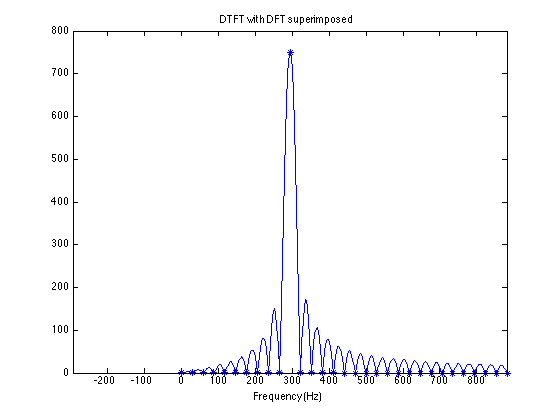
You can see that most of the DFT samples happen to line up precisely at the zeros of the DTFT.
Using a longer signal
Finally, let's look at what happens when you use a longer signal. (Joe said, "Can't I make the spread go away by using a sufficiently large number of samples of the sinusoid?" The answer, as we'll see demonstrated, is that you can make the spread get smaller, but you can't make it go away entirely as long as you have a finite number of samples.) Let's go up a factor of 10, to 15,000 samples of the sinusoid. (And let's go back to the original frequency of 307 Hz.)
f0 = 307;
M = 15000;
w0 = 2*pi*f0/Fs;
n = 0:(M-1);
y = cos(w0*n);
Y = fft(y);

M10 = length(y)*10;
Y10 = fft(y,M10);
f10 = (0:(M10-1))*Fs/M10;
f = (0:(M-1))*Fs/M;

plot(f10,abs(Y10));
hold on
plot(f,abs(Y),'*')
hold off

xlim([f1 f2])

title('DTFT with DFT superimposed')
xlabel('Frequency (Hz)')

The plot above is shown at the same scale as the one for M = 1500 further up. You can see that the peak is much narrower, but it's hard to see the details. Let's zoom in closer.
p = 2*Fs/(M+1);
f1 = f0 - 10*p;
f2 = f0 + 10*p;
xlim([f1 f2])

Now you can see that the DTFT shape and DFT samples look very much like what we got for the 1500-point windowed sinusoid. The width of the peak, as well as the spacing of the sidelobes, has been reduced by a factor of 10 (15000 / 1500). And the spacing (in Hz) of the DFT samples has been reduced by the same amount.
Summary
In summary, the Fourier transform of a finite portion of a sinusoid has a characteristic shape: a central peak (the "main lobe") with a bunch of "side lobes" in either direction from the peak. The DFT simply samples this shape. Depending on the exact frequency, the output of the DFT might look a little different, depending on where the frequency happens to line up with the DFT frequency bins.
- カテゴリ:
- Fourier transforms


コメント
コメントを残すには、ここ をクリックして MathWorks アカウントにサインインするか新しい MathWorks アカウントを作成します。