
Steer Beams to Reality: from Phased Array to Beamforming
In today’s post, Liping from the Student Programs Team will share her experience on how MATLAB and Simulink can help students to understand wireless communication theories on beamforming and precoding. Let us see what she is going to share.
When I took the course “Fundamentals of Wireless Communications”, I felt it was so hard to concentrate in the classes since the course material was filled with mathematics including matrices, stochastic processes, formula derivations, etc. After working on wireless communication systems such as LTE and 5G for many years, I found understanding the basic concepts and theories was so important since they are fundamental to different applications.
Many examples and reference applications in MATLAB can help you to understand complex wireless communication theories. In this script, I will show how a demo can help you to understand beamforming, a technique that has been widely used in 5G and even in 6G, radar, sonar, medical imaging, and audio array systems.
Table of Contents
What are Phased Arrays?
How to do Beamforming?
Line-of-Sight Channel
Multipath Channel
Summary
Further Exploration
Helper Functions
What are Phased Arrays?
To understand beamforming, you first need to know what beams are and how they are formed. Briefly, a beam pattern can be formed by a phased array, which refers to multiple elements that can measure or emit waves. The elements are arranged in some configuration and act together to produce a desired beam pattern. You can steer the beams by adjusting the phase of the signals to each element without physically moving the array. For more details, please watch Brian Douglas’ video “What are Phased Arrays?“, where he uses a lot of animations to explain the concept.
In wireless communications, the elements of a phased array could be antennas. From the snapshots below of Douglas’ video, you can see in the right figure that the beams of a Uniform Linear Array (ULA) of isotropic antennas, where signals from each antenna have been superimposed so the signal strength has been enhanced in some directions, while they have been canceled in the other directions.
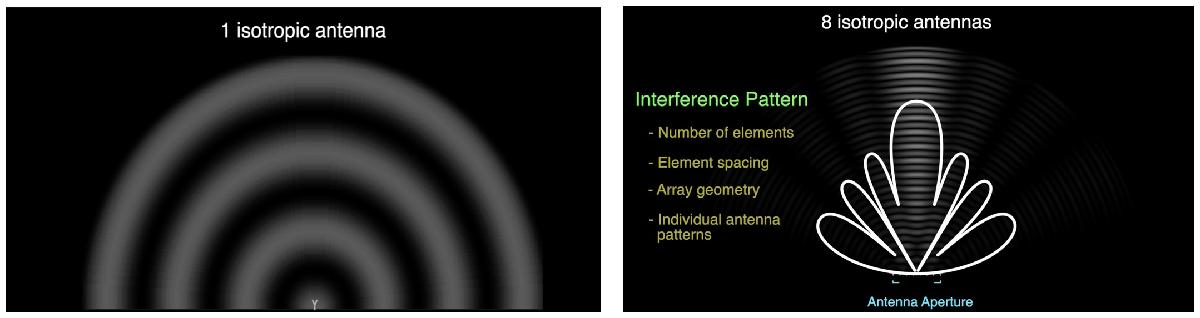
The beam pattern of an antenna array depends on the settings including the number of antenna elements, spacing between elements, array geometry as well as individual antenna patterns.
The Sensor Array Analyzer App in MATLAB provides you with an interactive tool to set up an antenna array, get its basic performance characteristics, and visualize its beam pattern in a 2D or 3D space. After installing the Phased Array Toolbox in MATLAB, you can find the Sensor Array Analyzer by going to the App Tab in the MATLAB Toolstrip, followed by searching under ‘Signal Processing and Communications’. You also can open the App with the following command in the MATLAB Command Window.
sensorArrayAnalyzer
When looking through the following example on how to use the Sensor Array Analyzer, you notice the App can help with tuning parameters, visualizing the beam pattern of a phased array, as well as steering a phased array to a certain direction. With different steering vectors, you can move beams around without moving the array physically.
Now you may still be curious about how to use beam steering to improve the performance of a wireless communication system. The answer is by beamforming, a scheme to pre-steer beams to a desired direction! The next example will show you how to do beamforming of an antenna array to improve the Signal-to-Noise Ratio (SNR) of a wireless link.
How to do Beamforming?
Antenna arrays have become part of the standard configuration in 5G. Such wireless communication systems are often referred to as Multiple-Input-and-Multiple-Output (MIMO) systems. To show the advantages of multiple antennas, we assume a wireless link deployed at 60 GHz, a millimeter wave frequency that had been newly considered in 5G.
close all; clear; clc;
rng(0); % set the seed of the random number generator
c = 3e8; % propagation speed
fc = 60e9; % carrier frequency
lambda = c/fc; % wavelength
With no loss in generality, we place a transmitter at the origin and a receiver approximately 1.6 km away.
txcenter = [0;0;0]; % center of the transmitter
rxcenter = [1500;500;0]; % center of the receiver
Then the Angle of Departure (AoD) and the Angle of Arrival (AoA) can be calculated based on the center locations of the transmitter and the receiver.
[~,txang] = rangeangle(rxcenter,txcenter); % AoD
[~,rxang] = rangeangle(txcenter,rxcenter); % AoA
Next, we consider two representive channel types.
Line-of-Sight Channel
Line-of-Sight (LOS) propagation is the simplest wireless channel that often happened in rural areas. Does adopting an antenna array under LOS propagation can increase the SNR at the receiver and thus improve the link’s bit error rate (BER)?
As a benchmark, you could simulate the BER performance of a Single-Input-and-Single-output (SISO) link under a LOS channel as follows, where the scatteringchanmtx function is used to create a channel matrix for different transmit and receive array configurations. The function simulates multiple scatterers between the transmit and the receive arrays assuming the signal travels from the transmit array to all the scatterers first and then bounces off the scatterers and arrives at the receive array. In this case, each scatterer defines a signal path between the transmit and the receive array, so the resulting channel matrix describes a multipath environment. You can read the details of this function by selecting it and then right-clicking to open the function.
Consider a SISO communication link where both the transmitter and the receiver only have a single antenna located at the node center, and there is a direct path from the transmitter to the receiver. Such a LOS channel can be modeled as a special case of a multipath environment.
txsipos = [0;0;0]; % antenna position to the transmitter
rxsopos = [0;0;0]; % antenna position to the receiver
g = 1; % path gain
sisochan = scatteringchanmtx(txsipos,rxsopos,txang,rxang,g); % generate a SISO LOS channel
Nsamp = 1e6; % sample rate
x = randi([0 1],Nsamp,1); % data source
ebn0_param = -10:2:10; % SNRs, unit in dB
Nsnr = numel(ebn0_param); % total number of SNRs
ber_siso = helperMIMOBER(sisochan,x,ebn0_param)/Nsamp; % caculate the bit error rate (BER)
You have got the BER performance of a SISO LOS link. When looking into the details of the helperMIMOBER function given in the Helper Functions session at the end of this script, you should notice BPSK modulation is considered in all the cases.
Now consider a MIMO link. we assume both the transmitter and the receiver are 4-element ULAs with half-wavelength spacing,
Ntx = 4; % number of transmitting antennas
Nrx = 4; % number of receiving antennas
txarray = phased.ULA(‘NumElements’,Ntx,‘ElementSpacing’,lambda/2); % antenna array of the transmitter
txmipos = getElementPosition(txarray)/lambda;
rxarray = phased.ULA(‘NumElements’,Nrx,‘ElementSpacing’,lambda/2); % antenna array of the receiver
rxmopos = getElementPosition(rxarray)/lambda;
With the receive antenna array, the received signals across array elements of the receiver are coherent, so it is possible to pre-steer the receive array toward the transmitter to improve the SNR. Moreover, the transmitter also can pre-steer the main beam of its antenna array toward the receiver for further improvement.
txarraystv = phased.SteeringVector(‘SensorArray’,txarray,…
‘PropagationSpeed’,c);
rxarraystv = phased.SteeringVector(‘SensorArray’,rxarray,…
‘PropagationSpeed’,c);
wt = step(txarraystv, fc, txang)’;
wr = conj(step(rxarraystv, fc, rxang));
mimochan = scatteringchanmtx(txmipos,rxmopos,txang,rxang,g);
ber_mimo = helperMIMOBER(mimochan,x,ebn0_param,wt,wr)/Nsamp;
helperPlotSpatialMIMOScene(txmipos,rxmopos,txcenter,rxcenter,NaN,wt,wr)
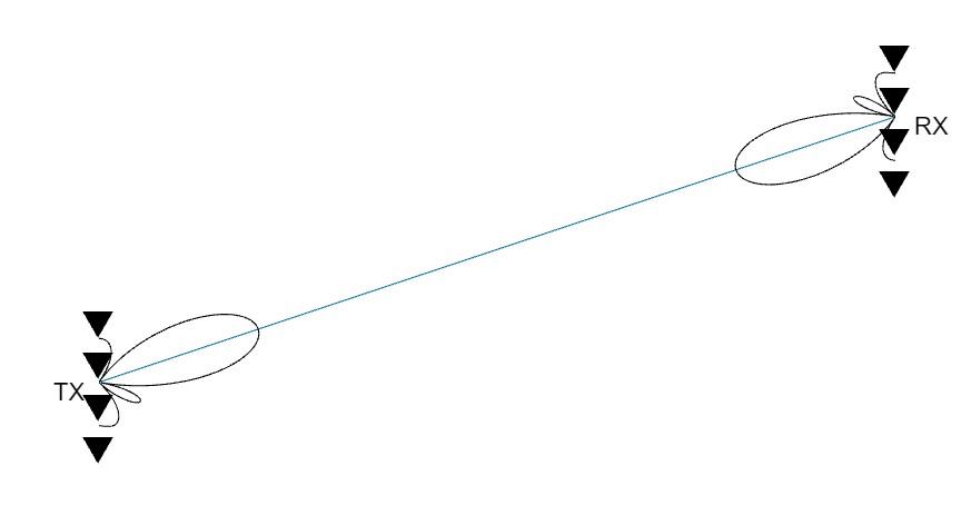
With beamforming, the modulated signal needs to be multiplied with wt before sending out at the transmitter, while the received signal needs to be multiplied with wr before demodulation at the receiver. After using the helperPlotSpatialMIMOScene function to visualize the scene in the figure above, you notice the main beams at the transmitter and the receiver have been pointed at each other.
Now you can compare the BER performance in the SISO and the MIMO cases under the LOS propagation channel,
helperBERPlot(ebn0_param,[ber_siso(:) ber_mimo(1,:).’]);
legend(‘SISO LOS’,‘MIMO LOS’);
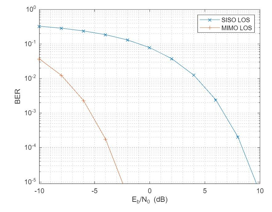
The BER curve shows the transmit array and the receive array contribute around 6 dB array gain respectively, resulting in a total gain of 12 dB over the SISO case.
Note that the gain is achieved under the assumption that the transmitter needs to know the receiver’s direction or location, and meanwhile the signal incoming direction is known to the receiver, where the angle is often obtained using the direction of arrival estimation algorithms.
Multipath Channel
In most cases, wireless communications occur in a multipath fading environment. The rest of this example explores how phased arrays can help in such a case.
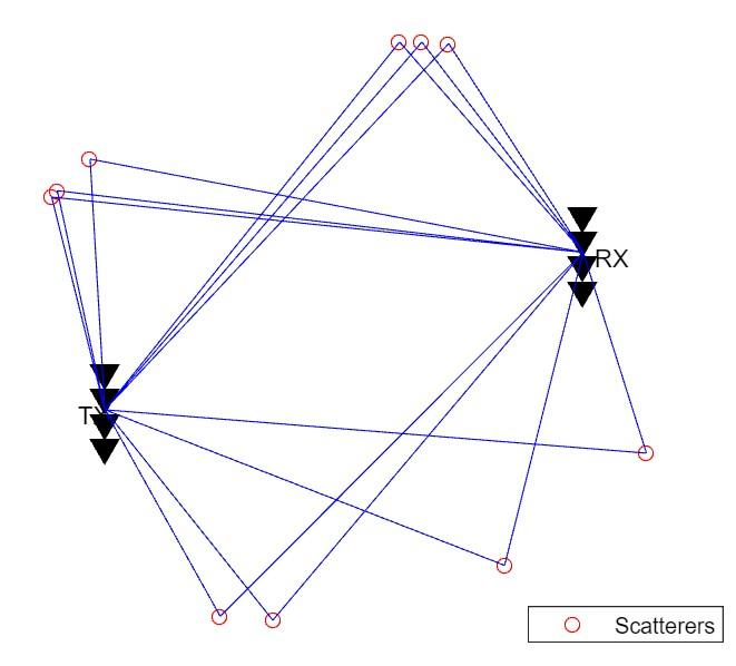
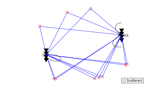
Assume there are 10 randomly placed scatterers in the channel, so there will be 10 paths from the transmitter to the receiver, as illustrated in the following.
Nscat = 10; % number of scatterers
[~,~,scatg,scatpos] = helperComputeRandomScatterer(txcenter,rxcenter,Nscat);
helperPlotSpatialMIMOScene(txmipos,rxmopos,txcenter,rxcenter,scatpos)
For simplicity, assume that signals traveling along all paths arrive within the same symbol period, so the channel is frequency flat and not frequency selective.
In such a multipath fading channel, the channel needs to change over multiple time slots to simulate the BER curve. Assume the simulation lasts 1000 frames and each frame has 10000 bits. The BER curve of the baseline SISO link under a multipath channel can be simulated as follows.
Nframe = 1e3; % number of frames
Nbitperframe = 1e4; % number of bits per frame
Nsamp = Nframe*Nbitperframe; % total number of data samples
x = randi([0 1],Nbitperframe,1); % generated the source data
nerr = zeros(1,Nsnr);
for m = 1:Nframe
sisompchan = scatteringchanmtx(txsipos,rxsopos,Nscat);
wr = sisompchan’/norm(sisompchan);
nerr = nerr + helperMIMOBER(sisompchan,x,ebn0_param,1,wr);
end
ber_sisomp = nerr/Nsamp;
In SISO cases, if you compare the channel matrix of a LOS channel with that of a multipath channel, you can notice it contains a single element and the value of the element changes from a real number to a complex number due to multipath fading. In such a case, a combining weight calculated as wr = sisompchan’/norm(sisompchan) can be used at the receiver to improve the SNR.
In the MIMO case, the BER curve can be simulated as follows, where the diagbfweights function is used to calculate the precoding weight wp at the transmitter and the combining weights wc at the receiver. You can right-click on the function and open it to see its details.
x = randi([0 1],Nbitperframe,Ntx);
nerr = zeros(Nrx,Nsnr);
for m = 1:Nframe
mimompchan = scatteringchanmtx(txmipos,rxmopos,Nscat);
[wp,wc] = diagbfweights(mimompchan);
nerr = nerr + helperMIMOBER(mimompchan,x,ebn0_param,wp,wc);
end
ber_mimomp = nerr/Nsamp;
To understand how precoding and combining weights are calculated, you first need to understand what Singular Value Decomposition (SVD) is. Use the following command to find the MATLAB documentation on SVD.
help svd
Briefly, an SVD ([U,S,V] = svd(X)) produces a diagonal matrix S, of the same dimension as X and with nonnegative diagonal elements in decreasing order, and unitary matrices U and V so that X = U*S*V’. Try following commands in MATLAB.
bf = wp*mimompchan*wc
[u,s,v] = svd(mimompchan)
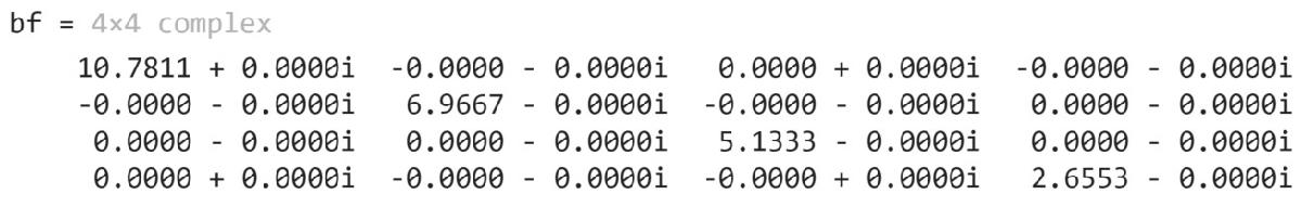
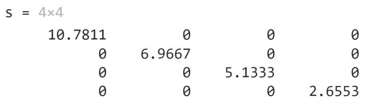
Compare bf with s, you now know the diagbfweights function is based on SVD. Due to a rich scatterer environment, the channel matrix of a MIMO multipath channel usually has full rank.
Note that the product wp*mimompchan*wc is a diagonal matrix, which means that the information received by each receive array element is simply a scaled version of the transmit array element. Such a MIMO multipath channel behaves like multiple orthogonal subchannels within the original channel.
Therefore, it is possible to send multiple data streams simultaneously across the MIMO multipath channel, which is called spatial multiplexing. The basic idea of spatial multiplexing is to separate the channel matrix into multiple modes so that the data stream sent from different elements in the transmit array can be independently recovered from the received signal. The goal of spatial multiplexing is less about increasing the SNR and more about increasing the information throughput.
Now you can plot the BER curves of the SISO multipath case, and the first two data streams in the MIMO multipath case. As a benchmark, you also plot the BER curve in the SISO LOS case that has been got from the previous section.
helperBERPlot(ebn0_param,[ber_siso(:) ber_sisomp(:) ber_mimomp(1,:).’ ber_mimomp(2,:).’]);
legend(‘SISO LOS’,‘SISO Multipath’,‘MIMO Multipath Stream 1’,‘MIMO Multipath Stream 2’);
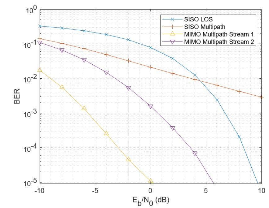
Compared to the BER curve of the SISO LOS channel, the BER curve of the SISO multipath channel falls off much slower due to the fading caused by the multipath propagation. Meanwhile, in the MIMO multipath case, the first subchannel corresponds to the dominant transmit and receive directions so there is no loss in the diversity gain, which refers to the gain on the slope change. Although the second stream cannot provide a gain as high as the first stream as it uses a less dominant subchannel, the overall information throughput can be improved since it is now possible to transmit multiple data streams simultaneously.
Summary
This demo explains how array processing can improve the performance of a MIMO wireless communication system. Depending on the nature of the channel, the arrays can be used to either improve the SNR via array gain or diversity gain; or improve the capacity via spatial multiplexing.
Now you understand some basics of MIMO wireless communications such as beamforming, precoding, diversity gain, and spatial multiplexing. The helper functions used in this demo are attached at the end of this script. Please run the code and reach out to us at studentcompetitions@mathworks.com if you have any further questions.
Further Exploration
Besides intuitively uniformly splitting the power among transmit elements, the capacity of the channel can be further improved by a water-filling algorithm. For details, please refer to the demo “Improve SNR and Capacity of Wireless Communication Using Antenna Arrays”.
To learn how to make beamforming real in 5G, please watch the tutorial video “Beamforming for MU-MIMO in 5G New Radio“. Moreover, a lot of examples and reference applications are available in the documentation on wireless communications, which can help you to understand the relevant concepts and theories more easily and clearly. Various examples of AI for Wireless can also provide you with more reference applications on how to apply AI technology in wireless communications. Have fun!
Helper Functions
The first helper function is for plotting the MIMO scene in a 2D area.
function helperPlotSpatialMIMOScene(txarraypos,rxarraypos,txcenter,rxcenter,scatpos,wt,wr)
narginchk(5,7);
rmax = norm(txcenter-rxcenter);
if size(txarraypos,2) == 1 && size(rxarraypos,2) == 1
spacing_scale = 0;
elseif size(txarraypos,2) == 1
spacing_scale = rmax/20/mean(diff(rxarraypos(2,:)));
else
spacing_scale = rmax/20/mean(diff(txarraypos(2,:)));
end
txarraypos_plot = txarraypos*spacing_scale+txcenter;
rxarraypos_plot = rxarraypos*spacing_scale+rxcenter;
figure
hold on;
plot(txarraypos_plot(1,:),txarraypos_plot(2,:),‘kv’,‘MarkerSize’,10,…
‘MarkerFaceColor’,‘k’);
text(txcenter(1)-85,txcenter(2)-15,‘TX’);
plot(rxarraypos_plot(1,:),rxarraypos_plot(2,:),‘kv’,‘MarkerSize’,10,…
‘MarkerFaceColor’,‘k’);
text(rxcenter(1)+35,rxcenter(2)-15,‘RX’);
if isnan(scatpos)
set(gca,‘DataAspectRatio’,[1,1,1]);
line([txcenter(1) rxcenter(1)],[txcenter(2) rxcenter(2)]);
else
hscat = plot(scatpos(1,:),scatpos(2,:),‘ro’);
for m = 1:size(scatpos,2)
plot([txcenter(1) scatpos(1,m)],[txcenter(2) scatpos(2,m)],‘b’);
plot([rxcenter(1) scatpos(1,m)],[rxcenter(2) scatpos(2,m)],‘b’);
end
legend(hscat,{‘Scatterers’},‘Location’,‘SouthEast’);
end
if nargin > 5
nbeam = rmax/5;
if ~isnan(wt)
txbeam_ang = -90:90;
txbeam = abs(wt*steervec(txarraypos,txbeam_ang)); % wt row
txbeam = txbeam/max(txbeam)*nbeam;
[txbeampos_x,txbeampos_y] = pol2cart(deg2rad(txbeam_ang),txbeam);
plot(txbeampos_x+txcenter(1),txbeampos_y+txcenter(2),‘k’);
end
if ~isnan(wr)
rxbeam_ang = [90:180 -179:-90];
rxbeam = abs(wr.’*steervec(rxarraypos,rxbeam_ang)); % wr column
rxbeam = rxbeam/max(rxbeam)*nbeam;
[rxbeampos_x,rxbeampos_y] = pol2cart(deg2rad(rxbeam_ang),rxbeam);
plot(rxbeampos_x+rxcenter(1),rxbeampos_y+rxcenter(2),‘k’);
end
end
axis off;
hold off;
end
The second helper function is for calculating the BER values of a MIMO link.
function nber = helperMIMOBER(chan,x,snr_param,wt,wr)
Nsamp = size(x,1);
Nrx = size(chan,2);
Ntx = size(chan,1);
if nargin < 4
wt = ones(1,Ntx);
end
if nargin < 5
wr = ones(Nrx,1);
end
xt = 1/sqrt(Ntx)*(2*x-1)*wt; % map to bpsk
nber = zeros(Nrx,numel(snr_param),‘like’,1); % real
for m = 1:numel(snr_param)
n = sqrt(db2pow(-snr_param(m))/2)*(randn(Nsamp,Nrx)+1i*randn(Nsamp,Nrx));
y = xt*chan*wr+n*wr;
xe = real(y)>0;
nber(:,m) = sum(x~=xe);
end
end
In the first two functions, a SISO scene/link can be considered as a special case of a MIMO scene/link.
The third function is for calculating the position of the scatterers.
function [txang,rxang,g,scatpos] = …
helperComputeRandomScatterer(txcenter,rxcenter,Nscat)
ang = 90*rand(1,Nscat)+45;
ang = (2*(rand(1,numel(ang))>0.5)-1).*ang;
r = 1.5*norm(txcenter-rxcenter);
scatpos = phased.internal.ellipsepts(txcenter(1:2),rxcenter(1:2),r,ang);
scatpos = [scatpos;zeros(1,Nscat)];
g = ones(1,Nscat);
[~,txang] = rangeangle(scatpos,txcenter);
[~,rxang] = rangeangle(scatpos,rxcenter);
end
The fourth function is for plotting BER curves.
function helperBERPlot(ebn0,ber)
figure
h = semilogy(ebn0,ber);
set(gca,‘YMinorGrid’,‘on’,‘XMinorGrid’,‘on’);
markerparam = {‘x’,‘+’,‘^’,‘v’,‘.’};
for m = 1:numel(h)
h(m).Marker = markerparam{m};
end
xlabel(‘E_b/N_0 (dB)’);
ylabel(‘BER’);
end
- カテゴリ:
- MATLAB


コメント
コメントを残すには、ここ をクリックして MathWorks アカウントにサインインするか新しい MathWorks アカウントを作成します。