
Deep Learning for Automated Driving (Part 1) – Vehicle Detection
This is a guest post from Avinash Nehemiah, Avi is a product manager for computer vision and automated driving.
 I often get questions from friends and colleagues on how automated driving systems perceive their environment and make “human-like” decisions and how MATLAB is used in these systems.
Over the next two blog posts I’ll explain how deep learning and MATLAB are used to solve two common perception tasks for automated driving:
I often get questions from friends and colleagues on how automated driving systems perceive their environment and make “human-like” decisions and how MATLAB is used in these systems.
Over the next two blog posts I’ll explain how deep learning and MATLAB are used to solve two common perception tasks for automated driving:
- Vehicle detection (this post)
- Lane detection (next post)
Vehicle Detection
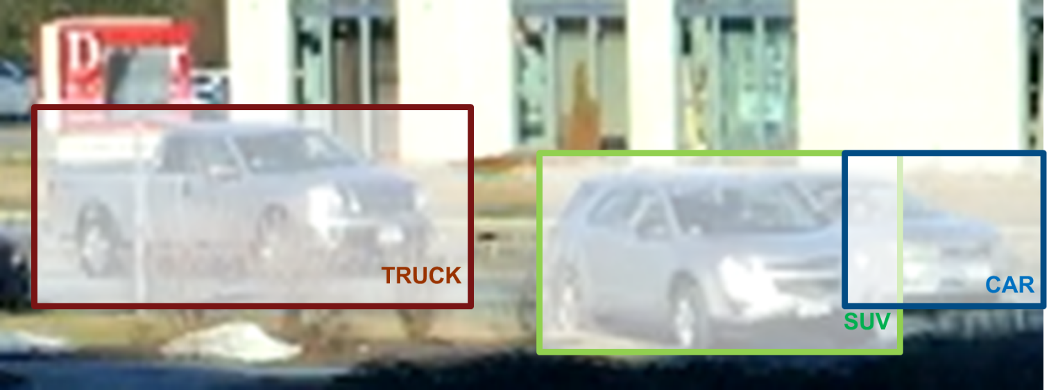
Object detection is the process of locating and classifying objects in images and video. In this section I’ll use a vehicle detection example to walk you through how to use deep learning to create an object detector. The same steps can be used to create any object detector. The figure below shows the output of a three class vehicle detector, where the detector locates and classifies each type of vehicle.
Output of a vehicle detector that locates and classifies different types of vehicles.
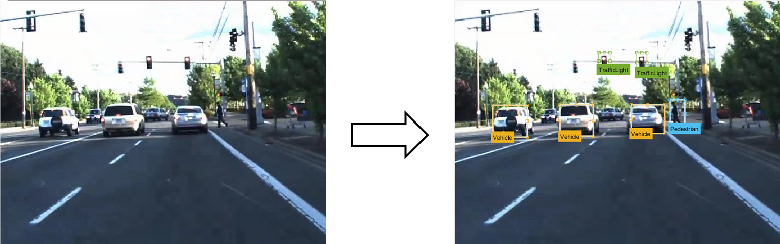
Before I can start creating a vehicle detector I need a set of labeled training data, which is a set of images annotated with the locations and labels of objects of interest. More specifically, someone needs to sift through every image or frame of video and label the locations of all objects of interest. This process is known as ground truth labeling. Ground truth labeling is often the most time-consuming part of creating an object detector. The figure below shows a raw training image on the left, and the same image with the labeled ground truth on the right.
Raw input image (left) and input image with labeled ground truth (right).
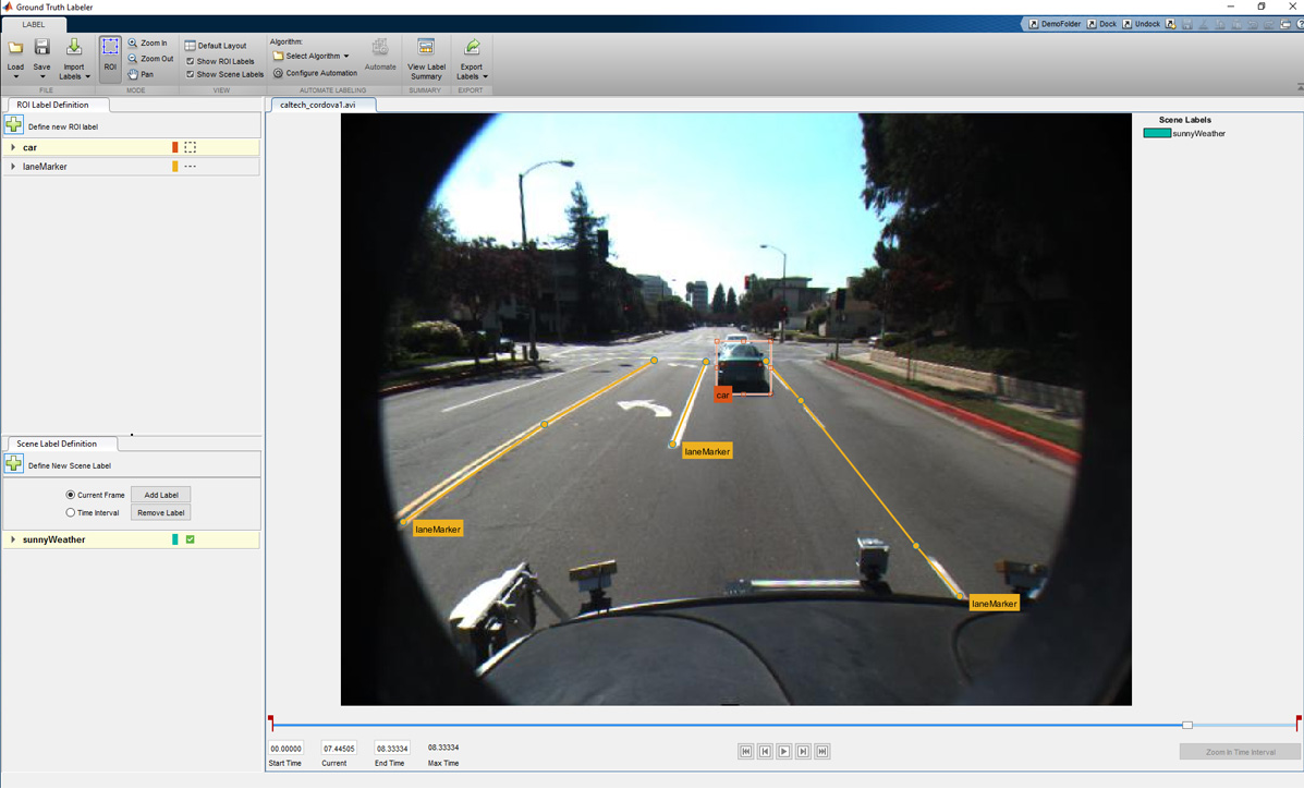
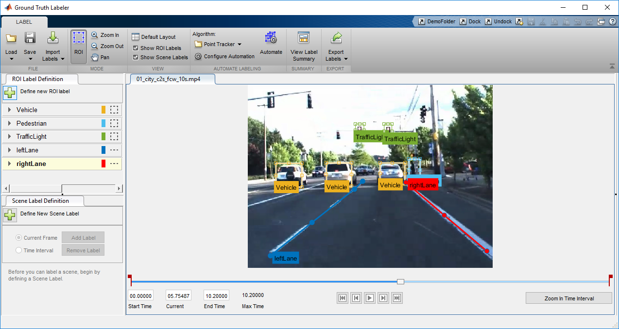
As you can imagine, labeling a sufficiently large set of training images can be a laborious and manual process. To reduce the amount of time I spend labeling data, I used the Ground Truth Labeler in Automated Driving System Toolbox, which is an app to label ground truth as well as automate part of the labeling process.
Screen shot of Ground Truth Labeler app designed to label video and image data.
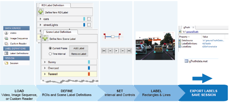
One way to automate part of the process is to use a tracking algorithm. The tracker I use is the Kanade Lucas Tomasi algorithm (KLT) which is one of the first computer vision algorithms to be used in real-world applications. The KLT algorithm represents objects as a set of feature points and tracks their movement from frame to frame. This lets us manually label one or more objects in the first frame, and use the tracker to label the rest of the video. The Ground Truth Labeler app also allows users to import their own algorithms to automate labeling. The most common way I’ve seen this feature used is when users import their own existing detectors to label new data, which helps them eventually create more accurate detectors. The figure below illustrates the workflow used to label a sequence of images or a video using the Ground Truth Labeler app.
Process of automating ground truth labeling using MATLAB.
The labeled data is stored as a table that lists the location of the vehicles in each time step of video from our training set. With the ground truth labeling complete, I can start training a vehicle detector. In our case I estimate the ground truth labeling process was sped up by up to 119x. The training video data for our video was captured at 30 frames per second, and we labeled objects every 4 seconds. That means we saved the time it would take to label the 119 frames in between. This 119x savings is a best case as we sometimes had to correct the output of the automated labeling. For our vehicle detector, I use a Faster R-CNN network. Let’s start by defining a network architecture as illustrated in the MATLAB code snippets below. The Faster R-CNN algorithm analyzes regions of an image and therefore the input layer is smaller than the expected size of an input image. In our case I choose a 32x32 pixel window. The input size is a balance between execution time and the amount of spatial detail you want the detector to resolve.% Create image input layer. inputLayer = imageInputLayer([32 32 3]);The middle layers are the core building blocks of the network, with repeated sets of convolution, ReLU and pooling layers. For our example, I’ll use just a couple of layers. You can always create a deeper network by repeating these layers to improve accuracy or if you want to incorporate more classes into the detector. You can learn more about the different types of layers available in the Neural Network Toolbox documentation.
% Define the convolutional layer parameters.
filterSize = [3 3];
numFilters = 32;

% Create the middle layers.
middleLayers = [
convolution2dLayer(filterSize, numFilters, 'Padding', 1)
reluLayer()
convolution2dLayer(filterSize, numFilters, 'Padding', 1)
reluLayer()
maxPooling2dLayer(3, 'Stride',2)
];
The final layers of a CNN are typically a set of fully connected layers and a softmax loss layer. In this case, I’ve added a ReLU nonlinearity between the fully connected layers to improve detector performance since our training set for this detector wasn’t as large as I would like.
finalLayers = [
% Add a fully connected layer with 64 output neurons. The output size
% of this layer will be an array with a length of 64.
fullyConnectedLayer(64)
% Add a ReLU non-linearity.
reluLayer()
% Add the last fully connected layer. At this point, the network must
% produce outputs that can be used to measure whether the input image
% belongs to one of the object classes or background. This measurement
% is made using the subsequent loss layers.
fullyConnectedLayer(width(vehicleDataset))
% Add the softmax loss layer and classification layer.
softmaxLayer()
classificationLayer()
];

layers = [
inputLayer
middleLayers
finalLayers
]
To train the object detector, I pass the "layers" network structure to the "trainFasterRCNNObjectDetector" function. If you have a GPU installed, the algorithm will default to using the GPU. If you want to train without a GPU or use multiple GPUs, you can do so by adjusting the "ExecutionEnvironment" parameter in "trainingOptions".
detector = trainFasterRCNNObjectDetector(trainingData, layers, options, ...
    'NegativeOverlapRange', [0 0.3], ...
    'PositiveOverlapRange', [0.6 1], ...
    'BoxPyramidScale', 1.2);
Once training is done, try it out on a few test images to see if the detector is working properly. I used the following code to test the detector on a single image.
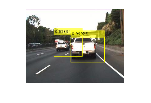
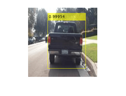
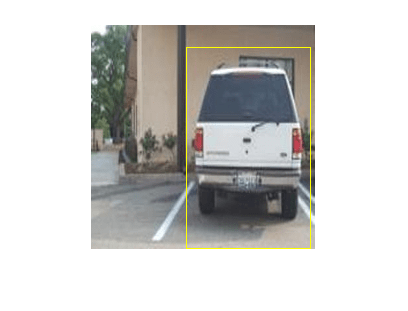
% Read a test image.
 I = imread('highway.png');

 % Run the detector.
 [bboxes, scores] = detect(detector, I);

 % Annotate detections in the image.
 I = insertObjectAnnotation(I, 'rectangle', bboxes, scores);
 figure
 imshow(I)
Detected bounding boxes and scores from Faster R-CNN vehicle detector.
Once you are confident that your detector is working, I highly recommend testing it on a larger set of validation images using a statistical metric such as average precision which provides a single score measure of the ability of the detector to make correct classifications (precision) and the ability of the detector to find all relevant objects (recall). This page provides more information on how you can evaluate a detector. To solve the problems described in this post I used MATLAB R2017b along with Neural Network Toolbox, Parallel Computing Toolbox, Computer Vision System Toolbox, and Automated Driving System Toolbox.- 类别:
- Deep Learning


评论
要发表评论,请点击 此处 登录到您的 MathWorks 帐户或创建一个新帐户。