
Open AI Caribbean Data Science Challenge
The following post is from Neha Goel, Champion of student competitions and online data science competitions. She's here to promote a new Deep Learning challenge available to everyone. If you win, you get money, plus a bonus if you use MATLAB. Read on!
Hello all! We at MathWorks, in collaboration with DrivenData, are excited to bring you this challenge. Through this challenge you'll be working with a real-world dataset of drone aerial imagery (big images) for classification. The competition link is here.
The prizes are:
The bonus is for the best solution specifically using MATLAB. The competition ends Dec 23rd, 2019 at midnight.
| Place | Prize Amount |
|---|---|
| 1st | $5,000 |
| 2nd | $2,000 |
| 3rd | $1,000 |
| Bonus | $2,000 |
The premise is simple: given aerial imagery, can you correctly identify roof material of individual structures? This challenge focuses on the disaster risk management of cities which are prone to natural hazards. You are provided with large aerial images captured by drones of regions in Colombia, St. Lucia, and St. Guatemala. The data includes aerial imagery and GeoJSON files including the building footprint, unique building ID, and roof material labels (for the training data).
The dataset is around 30GB in total. Within it there are 3 folders for each country - Colombia, Guatemala, and St. Lucia. Each country's folder consists of subfolders of areas/regions. For instance, within "Colombia" we have 2 regions named "borde_rural" and "borde_soacha". Each region's folder has:
- A BigTIFF image file of the region -- for example, borde_rural_ortho-cog.tif
- GeoJSON files with metadata on the image extent in latitude/longitude, training data, and test data
Since we are sponsoring the competition, we are also providing a basic "starter code" in MATLAB: Not only how to build and train a basic classification model, but also extracting the individual structures based on lat/long metadata and saving the results as a CSV file in the format required for the challenge.
This should serve as basic code where you can start analyzing the data and work towards developing a more efficient, optimized, and accurate model using more of the training data available. What's nice is we've taken care of all the tedious parts for you: reading the input files, identifying the regions of interest and saving the results out to a file for submission. This MATLAB code is available for download here.
On the challenge's Problem Description page, all required details for images, features, labels and submission metrics are provided.
Next, I'll walk you through the code at a high level. If you're interested in getting the full walkthrough of the starter code: you can check out my in-depth blog on DrivenData's website: http://drivendata.co/blog/disaster-response-roof-type-benchmark/
LOADING AND PREPARING DATA
Load the data as a bigimage
bigimage is a new Image Processing Toolbox function in MATLAB R2019b for processing very large images that may not fit in memory. This function is very convenient for these large images. So here we are creating bigimage objects for the BigTIFF image of each region.
bimg = bigimage(which(regionNames(idx) + "_ortho-cog.tif"));
Split the image into the RGB channel and the mask
Inspecting the images, you realize quickly this has 4 channels: 3 channels of RGB and a 4th mask channel of opacity. With the use of the helper function separateChannels we are removing the opacity mask channel. For further training we will only be using the 3 RGB channels.brgb = apply(bimg,1, @separateChannels,'UseParallel',true);
Set the spatial reference for the bigimage
Since each region's image spans a rectangular region with a particular latitude and longitude extent, we want to assign this as the spatial reference for the image. This will allow us to extract image regions by using the latitude and longitude value rather than the pixel values, which we will need to do later.
For more information, refer to the Set Spatial Referencing for Big Images example in the documentation.
Create Training Data
The training set consists of 3 pieces of information that can be parsed from the GeoJSON files for each region
- The building ID
- The building polygon coordinates (in latitude-longitude points)
- The building material
To extract the training set, we are opening the GeoJSON file of each region, reading it, and decoding the files using the jsondecode function.
for idx = 1:numel(regionNames)
 fid = fopen("train-" + regionNames(idx) + ".geojson");
 trainingStructs(idx) = jsondecode(fread(fid,inf,'*char'));
 fclose(fid);
end
Extract the ID, material, and coordinates of each ROI, Increment the index of regions as we loop through the training set to ensure we are referring to the correct region,Correct for coordinate convention by flipping the Y image coordinates of the building region coordinates, Convert the text array of materials to a categorical array for later classification.

 Notice that the number of samples for each material can be quite different, which means the classes are not balanced. This could affect the performance of your model if you do not address this, since this may bias the model to predict materials that are more frequent in the training set.


regionIdx = 1;
for k = 1:numTrain
 trainID{k} = trainingStruct(k).id;
 trainMaterial{k} = trainingStruct(k).properties.roof_material;
 coords = trainingStruct(k).geometry.coordinates;
 if iscell(coords)
  coords = coords{1};
 end

 trainCoords{k} = squeeze(coords);
 if numTrainRegionsCumulative(regionIdx)
  regionIdx = regionIdx + 1;
 end
 trainCoords{k}(:,2) = brgb(regionIdx).SpatialReferencing(1).YWorldLimits(2)- ...
    (trainCoords{k}(:,2)-brgb(regionIdx).SpatialReferencing(1).YWorldLimits(1));

end
trainMaterial = categorical(trainMaterial);
Visualize the Training Data
We also provide ways to visualize the data to ensure you're grabbing the correct regions of interest. Using the function bigimageshow, the data looks like this:
EXPLORING THE DATA
Create Image Datastore from Saved Training Images
First we will create an imageDatastore for the training_data folder. This is used to manage a collection of image files, where each individual image fits in memory, but the entire collection of images does not necessarily fit.
To further augment and preprocess the data images we recommend looking at the following resources:
- Preprocess Images for Deep Learning
- Augment Images for Deep Learning Workflows Using Image Processing Toolbox
imds = imageDatastore("training_data","IncludeSubfolders",true, ...
 "FileExtensions",".png","LabelSource","foldernames")
Show a count of the distribution of all 5 materials.
labelInfo = countEachLabel(imds)
Notice that the number of samples for each material can be quite different, which means the classes are not balanced. This could affect the performance of your model if you do not address this, since this may bias the model to predict materials that are more frequent in the training set.
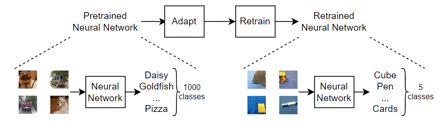
Configure Pretrained Network for Transfer Learning
In this example we use the ResNet-18 neural network as a baseline for our classifier. You can also use other networks to perform transfer learning.
NOTE: You will first have to download the Deep Learning Toolbox Model for ResNet-18 Network support package.
net = resnet18;
To retrain ResNet-18 to classify new images, replace the last fully connected layer and the final classification layer of the network. In ResNet-18, these layers have the names 'fc1000' and 'ClassificationLayer_predictions', respectively. Set the new fully connected layer to have the same size as the number of classes in the new data set. To learn faster in the new layers than in the transferred layers, increase the learning rate factors of the fully connected layer using the 'WeightLearnRateFactor' and 'BiasLearnRateFactor' properties.
numClasses = numel(categories(imds.Labels));
lgraph = layerGraph(net);

newFCLayer = fullyConnectedLayer(numClasses,'Name','new_fc','WeightLearnRateFactor',10,'BiasLearnRateFactor',10);
lgraph = replaceLayer(lgraph,'fc1000',newFCLayer);

newClassLayer = classificationLayer('Name','new_classoutput');
lgraph = replaceLayer(lgraph,'ClassificationLayer_predictions',newClassLayer);
View the modified network using the analyzeNetwork function. You can also open it using the Deep Network Designer app.
analyzeNetwork(lgraph);
Training Options
Configure the image datastore to use the neural network's required input image size. To do this, we are registering a custom function called readAndResize.
Split the training data into training and validation sets. Note that this is randomly selecting a split, but you may want to look into the splitEachLabel function for other options to make sure the classes are balanced
[imdsTrain,imdsVal] = splitEachLabel(imds,0.7,"randomized");
Specify the training options, including mini-batch size and validation data. Set InitialLearnRate to a small value to slow down learning in the transferred layers. In the previous step, you increased the learning rate factors for the fully connected layer to speed up learning in the new final layers. This combination of learning rate settings results in fast learning only in the new layers and slower learning in the other layers.
HINT: You can work with different options to improve the training. Check out the documentation for trainingOptions to learn more.
options = trainingOptions('sgdm', ...
 'MiniBatchSize',32, ...
 'MaxEpochs',5, ...
 'InitialLearnRate',1e-4, ...
 'Shuffle','every-epoch', ...
 'ValidationData',imdsVal, ...
 'ValidationFrequency',floor(numel(imdsTrain.Files)/(32*2)), ...
 'Verbose',false, ...
 'Plots','training-progress');
Train the Network
Here you will use the imagedatastores, layer graph, and training options to train your model.
Note that training will take a long time using a CPU. However, MATLAB will automatically detect if you have a supported GPU to help you accelerate training.
Set the doTraining flag below to false to load a presaved network.
doTraining = false;
if doTraining
 netTransfer = trainNetwork(imdsTrain,lgraph,options);
else
 load resnet_presaved.mat
end
 Note: this is starter code, with a final accuracy of less than 80%. We're not trying to win the competition with this code, it's up to you to improve it, submit and win!
Predict on the Test Set
Once we have our trained network, we can perform predictions on our test set. To do so, first we will create an image datastore for the test set.
imdsTest = imageDatastore("test_data","FileExtensions",".png");
Next we predict labels (testMaterial) and scores (testScores) using the trained network
NOTE: This will take some time, but just as with training the network, MATLAB will determine whether you have a supported GPU and significantly speed up this process.
[testMaterial,testScores] = classify(netTransfer,imdsTest)
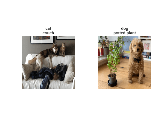
The following code will display the predicted materials for a few test images.
figure
displayIndices = randi(numTest,4,1);
for k = 1:numel(displayIndices)
 testImg = readimage(imdsTest,displayIndices(k));
 subplot(2,2,k)
 imshow(testImg);
 title(string(testMaterial(displayIndices(k))),"Interpreter","none")
end
Thanks for following along with this code! We are excited to find out how you will modify this starter code and make it yours. We strongly recommend looking at our Deep Learning Tips & Tricks page for more ideas on how you can improve our benchmark model.
Don't forget to visit the competition page to get started, and feel free to reach out to us in the DrivenData forum or email us at studentcompetitions@mathworks.com if you have any further questions.
- 범주:
- Deep Learning


댓글
댓글을 남기려면 링크 를 클릭하여 MathWorks 계정에 로그인하거나 계정을 새로 만드십시오.