The following post is by Dr. Barath Narayanan, University of Dayton Research Institute (UDRI) with co-authors: Dr. Russell C. Hardie, and Redha Ali.
In this blog, we apply Deep Learning based segmentation to skin lesions in dermoscopic images to aid in melanoma detection.
Affiliations:
*
Sensors and Software Systems, University of Dayton Research Institute, 300 College Park, Dayton, OH, 45469
**
Department of Electrical and Computer Engineering, University of Dayton, 300 College Park, Dayton, OH,
45469
Background
Skin lesion segmentation is an important step in Computer-Aided Diagnosis (CAD) of melanoma. In this blog, we present a Convolutional Neural Network (CNN) based segmentation approach applied to skin lesions in dermoscopic images. Early stage detection and diagnosis of melanoma detection increases one's survival rate significantly.
Please cite the following article if you're using any part of the code for your research.
[1]
Ali, R.,
Hardie, R. C.,
Narayanan, B. N., & De Silva, S. (2019, July). "
Deep learning ensemble methods for skin lesion analysis towards melanoma detection". In 2019 IEEE National Aerospace and Electronics Conference (NAECON) (pp. 311-316). IEEE.
Dataset utilized for this blog is taken from
ISIC 2018. Instructions about the dataset are provided at the end of this post.
Load the Dataset and Resize
| Raw images are loaded using imageDatastore. It is a computationally efficient function to collect image information. Load the ground truth masks using pixelLabelDatastore. White region in the ground truth mask indicates the "lesion" and rest of the image belongs to "background" class. The function pixelLabelImageDatastore helps in tagging the raw image with its corresponding ground truth mask. Let's visualize certain random images from the dataset for our reference. Later, resize all images to a size 224 x 224 for the deep learning network.
|
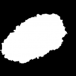 Labeled image showing pixels as either background (black) and foreground "lesion" (white) |
clear; close all; clc;
imds=imageDatastore('ISIC2018_Task1-2_Training_Input','IncludeSubfolders',true);
classNames=["Lesion","Background"];
labelIDs=[255,0];
pxds=pixelLabelDatastore('ISIC2018_Task1_Training_GroundTruth',classNames, labelIDs);
pximds=pixelLabelImageDatastore(imds,pxds);
total_num_images=length(pximds.Images);
perm=randperm(total_num_images,4);
figure;
for idx=1:length(perm)
[~,filename]=fileparts(pximds.Images{idx});
subplot(2,2,idx);
imshow(imread(pximds.Images{perm(idx)}));
hold on;
visboundaries(imread(pximds.PixelLabelData{perm(idx)}),'Color','r');
title(sprintf('%s',filename),'Interpreter',"none");
end

imageSize=[224 224 3];
pximdsResz=pixelLabelImageDatastore(imds,pxds,'OutputSize',imageSize);
clearvars -except pximdsResz classNames total_num_images imageSize
Split the Dataset - Training, Validation and Testing
test_idx=randperm(total_num_images,100);
train_valid_idx=setdiff(1:total_num_images,test_idx);
valid_idx=train_valid_idx(randperm(length(train_valid_idx),100));
train_idx=setdiff(train_valid_idx,valid_idx);
pximdsTrain=partitionByIndex(pximdsResz,train_idx);
pximdsValid=partitionByIndex(pximdsResz,valid_idx);
pximdsTest=partitionByIndex(pximdsResz,test_idx);
Deep Learning Approach
Define the CNN network for training the network along with the parameters necessary.
In this blog, we study the performance using DeepLab v3+ network. DeepLab v3+ is a CNN for semantic image segmentation. It utilizes an encoder-decoder based architecture with dilated convolutions and skip convolutions to segment images. In [1], we present an ensemble approach of combining both U-Net with DeepLab v3+ network. In the blog, we solely focus on DeepLab v3+ network using ResNet50 architecture. Feel free to change the hyperparameters and observe the performance.
Notes:
- Make sure to install Deep Learning Toolbox Model for ResNet-50 Network support package through add-on explorer.
- The input normalization might take about 5-10 minutes due to resolution of the original images. Training time per epoch is about 10 minutes in NVIDIA GeForce GTX 1070.
- You can also set the execution environment to 'multi-gpu' in the training options if you have access to more than one GPU.
numClasses=length(classNames);
lgraph=deeplabv3plusLayers(imageSize, numClasses,'resnet50');
options=trainingOptions('sgdm',...
'InitialLearnRate', 0.03, ...
'Momentum',0.9,...
'L2Regularization',0.0005,...
'MaxEpochs',20,...
'MiniBatchSize',32,...
'VerboseFrequency',20,...
'LearnRateSchedule','piecewise',...
'ExecutionEnvironment','gpu',...
'Shuffle','every-epoch',...
'ValidationData',pximdsValid, ...
'ValidationFrequency',50, ...
'ValidationPatience',4,...
'Plots','training-progress',...
'GradientThresholdMethod','l2norm',...
'GradientThreshold',0.05);
net=trainNetwork(pximdsTrain,lgraph,options);

Testing and Performance Analysis
Now, let's study the performance of the network on the test set. We study the performance in terms of following metrics:
- Pixel classification accuracy: global and mean
- Intersection over Union (IoU): weighted and mean
- Normalized confusion matrix
In [1], we also study the performance in terms of Jaccard index and Dice coefficient.
[pxdspredicted]=semanticseg(pximdsTest,net,'WriteLocation',tempdir);
metrics=evaluateSemanticSegmentation(pxdspredicted,pximdsTest);

normConfMatData=metrics.NormalizedConfusionMatrix.Variables;
figure
h=heatmap(classNames,classNames,100*normConfMatData);
h.XLabel='Predicted Class';
h.YLabel='True Class';
h.Title='Normalized Confusion Matrix (%)';

Visual Inspection
In this section, we visually inspect the results by visualizing both the predicted and actual masks for a given image.
num_test_images=length(pximdsTest.Images);
perm=randperm(num_test_images,2);
for idx=1:length(perm)
[~,filename]=fileparts(pximdsTest.Images{idx});
I=imread(pximdsTest.Images{perm(idx)});
I=imresize(I,[imageSize(1) imageSize(2)],'bilinear');
figure;
image(I);
hold on;
actual_mask=imread(pximdsTest.PixelLabelData{perm(idx)});
actual_mask=imresize(actual_mask,[imageSize(1) imageSize(2)],'bilinear');
visboundaries(actual_mask,'Color','r');
predicted_image=(uint8(readimage(pxdspredicted,perm(idx)))); % Values are 1 and 2
predicted_results=uint8(~(predicted_image-1)); % Conversion to binary and reverse the polarity to match with the labelIds
visboundaries(predicted_results,'Color','g');
title(sprintf('%s Red- Actual, Green - Predicted',filename),'Interpreter',"none");
imwrite(mat2gray(predicted_results),sprintf('%s.png',filename));
end


Conclusions
In this blog, we have presented a simple deep learning-based segmentation applied to skin lesions in dermoscopic images to aid in melanoma detection. The segmentation algorithm using DeepLab v3+ with ResNet50 architecture performed relatively well with a good IoU and pixel classification accuracy. Combining these results with other existing architectures would provide a boost in performance. Feel free to study the performance under different hyperparameters settings and architectures. In our paper [1], we fused the results of DeepLab v3+ with a U-Net architecture. Segmentation of skin lesion would serve as a valuable preprocessing step for classification algorithm for the detection of melanoma.
Dataset Instructions
Please cite the following articles if you're using the dataset.
[2] Noel Codella, Veronica Rotemberg, Philipp Tschandl, M. Emre Celebi, Stephen Dusza, David Gutman, Brian Helba, Aadi Kalloo, Konstantinos Liopyris, Michael Marchetti, Harald Kittler, Allan Halpern: “Skin Lesion Analysis Toward Melanoma Detection 2018: A Challenge Hosted by the International Skin Imaging Collaboration (ISIC)”, 2018; https://arxiv.org/abs/1902.03368
[3] Tschandl, P., Rosendahl, C. & Kittler, H. The HAM10000 dataset, a large collection of multi-source dermatoscopic images of common pigmented skin lesions. Sci. Data 5, 180161 doi:10.1038/sdata.2018.161 (2018).
Download the
ISIC 2018 Task 1,2 Training Data (10.4 GB) and the Training Ground Truth (26 MB) for Task 1. After downloading the zip files, extract them into respective folders ("ISIC2018_Task1-2_Training_Input", "ISIC2018_Task1_Training_GroundTruth" as needed for the script). The dataset contains 2594 images in total. Note that we solely utilize "Task 1 - Training Data" to study the performance of the system, as the ground truth is publicly available.
Biography
 |
Barath Narayanan graduated with M.S. and Ph.D. degree in Electrical Engineering from University of Dayton (UD) in 2013 and 2017 respectively. He currently holds a joint appointment as a Research Scientist at UDRI's Software Systems Group and as an Adjunct Faculty for the ECE department at UD. He graduated with distinction from SRM University, Chennai, India in 2012 with a Bachelor’s degree in Electrical and Electronics Engineering. His research interests include deep learning, machine learning, computer vision, and pattern recognition. |
 |
Redha Ali received his B.S. in Computer Science and Information Technology from the College of Electronic Technology, Bani Walid, Libya, in 2012. He completed his M.S. in Electrical and Computer Engineering from the University of Dayton in 2016. His Master's thesis work and publication are in the field of image and video denoising. He is currently pursuing his Ph. D. research in medical imaging at the University of Dayton. His applied research interests include medical image processing, deep learning, machine learning, computer vision, video restoration, and enhancement. |
 |
Dr. Russell C. Hardie graduated Magna Cum Laude from Loyola University in Baltimore Maryland in 1988 with a B.S. degree in Engineering Science. He obtained an M.S. and Ph.D. degree in Electrical Engineering from the University of Delaware in 1990 and 1992, respectively. Dr. Hardie served as a Senior Scientist at Earth Satellite Corporation (Now MDA) in Maryland prior to his appointment at the University of Dayton in 1993. He is currently a Full Professor in the Department of Electrical and Computer Engineering and holds a joint appointment with the Department of Electro-Optics and Photonics. |
Have a question or comment for the authors? Leave a comment below.


Comments
To leave a comment, please click here to sign in to your MathWorks Account or create a new one.