
What Is Physics-Informed Machine Learning?
This blog post is from Mae Markowski, Senior Product Manager at MathWorks.
Physics-informed machine learning is a branch of Scientific Machine Learning (SciML) that combines physical laws with machine learning and deep learning techniques. This integration is bi-directional: physics principles—such as conservation laws, governing equations, and other domain knowledge—inform artificial intelligence (AI) models, improving their accuracy and interpretability, while AI techniques can augment and even uncover governing equations and unknown model parameters, deepening our understanding of physical systems.
Physics-informed machine learning enables tasks such as predicting phenomena with greater precision and less data, as well as solving differential equations more efficiently. With MATLAB and Deep Learning Toolbox, you can develop AI models that leverage governing physics to enhance analysis and decision-making in engineering and science. In this blog, I will give you an overview of physics-informed machine learning: what it’s used for, what we mean by physics knowledge and how it informs AI methods, as well as benefits and promising applications of this exciting technology.
You can find relevant code and examples in the repository SciML and Physics-Informed Machine Learning Examples. In a future post, we’ll take a closer look at specific techniques for physics-informed machine learning.
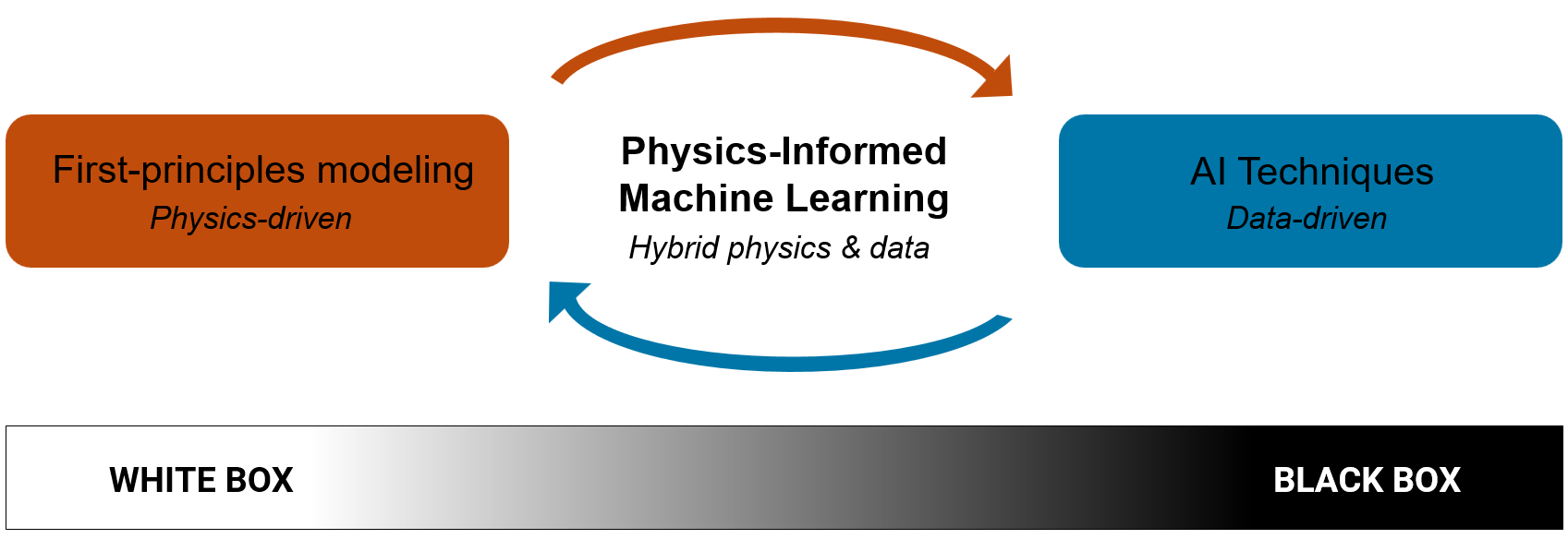 Figure: Physics-informed machine learning is a hybrid approach that combines the strengths of first-principles modeling (white box) with data-driven AI techniques (black-box).
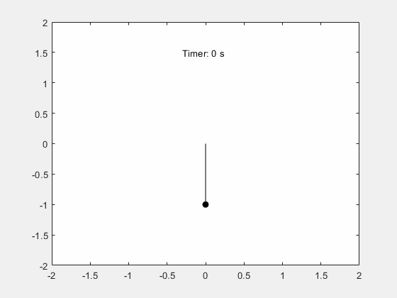 Figure: Simulation of a simple pendulum. To learn how to recreate this animation, see the example Simulate the Motion of the Periodic Swing of a Pendulum.
You might want to:
Figure: Simulation of a simple pendulum. To learn how to recreate this animation, see the example Simulate the Motion of the Periodic Swing of a Pendulum.
You might want to:
Table: Key objectives of physics-informed machine learning and illustrative examples using a simple pendulum
In the next blog post, we’ll dive deeper into the specific physics-informed machine learning techniques introduced above, along with a few others, and discuss their MATLAB implementations. For now, let’s explore what “physics” means in physics-informed machine learning, and how it can “inform” learning algorithms.
Table: Examples of how physics knowledge can be represented, illustrated with a simple pendulum. This list is not exhaustive—physics knowledge may also include symmetries, invariances, empirical relationships, and more.
For more information and examples on how domain knowledge can be integrated with machine learning, see Building Confidence in AI with Constrained Deep Learning and Use Physics-Inspired Estimators for Estimating Nonlinear Dynamics.
Table: Six stages of a traditional machine learning workflow
Physics can be incorporated at various stages of this workflow but often informs the model’s structure (stage 3) and evaluation (stage 4). Machine-learned components can also supplement physics-based models to address partially unknown dynamics (stage 1).
A key strategy in physics-informed machine learning is to impose constraints based on physics principles, ensuring predictions are not only accurate but also physically plausible. There are two main approaches for imposing constraints:
Table: Examples of physics-based constraints for the pendulum, and how they can be represented and enforced in deep learning models using MATLAB
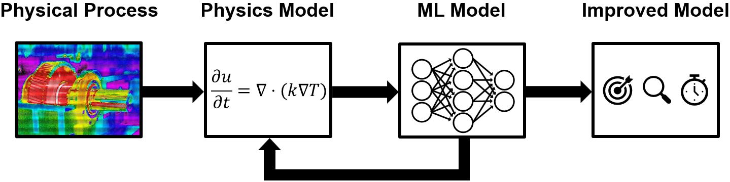 Figure: Physics-informed machine learning enhances AI models with known physics, or leverages AI to improve partially known physics models, resulting in methods that are more accurate, interpretable, and efficient.
Let’s look at some of the fields already benefiting from physics-informed machine learning.
Figure: Physics-informed machine learning enhances AI models with known physics, or leverages AI to improve partially known physics models, resulting in methods that are more accurate, interpretable, and efficient.
Let’s look at some of the fields already benefiting from physics-informed machine learning.
Figure: Physics-informed machine learning is a hybrid approach that combines the strengths of first-principles modeling (white box) with data-driven AI techniques (black-box).
What Is Physics-Informed Machine Learning Used for?
To illustrate the versatility of physics-informed machine learning, let’s use a familiar example: the pendulum. Imagine watching a pendulum swing, like the one below.
Figure: Simulation of a simple pendulum. To learn how to recreate this animation, see the example Simulate the Motion of the Periodic Swing of a Pendulum.
You might want to:
- Predict the pendulum’s future motion from data,
- Discover the underlying equations governing its swing, or
- Use a known equation to calculate its motion.
Modeling Unknown Dynamics
Consider a scenario where you have measurements of a pendulum’s angle and angular velocity over time. Suppose that the exact governing equation is unknown, but you do know that the total energy of the system is conserved. Certain physics-informed machine learning methods, such as Hamiltonian Neural Networks, allow you to build a model that learns from data and predicts the pendulum’s future swings, while accounting for energy conservation.Discovering Equations
Now imagine you want to discover an equation that describes the pendulum’s motion over time. Some physics-informed machine learning methods, like SINDy (Sparse Identification of Nonlinear Dynamics), can reveal the underlying mathematical relationships from data. For example, if you suspect there is unmodeled friction in the standard pendulum equation, these equation discovery techniques can be used to uncover a mechanistic model of the friction.Solving Known Equations
In cases where the governing equation is already known, you might want to combine it with experimental data to predict the pendulum’s angle over time or to solve the equation under different conditions, such as varying the forcing function. Methods like Physics-Informed Neural Networks can combine governing equations in the form of ordinary and partial differential equations (ODEs and PDEs) with data to find solutions that match both observed data and physical laws. Furthermore, if you have numerical solutions of the governing equations corresponding to different forcing functions, operator learning techniques like Fourier Neural Operator can be used to rapidly predict the solution (e.g. pendulum angle) given a new input (e.g. forcing function). Below is a summary of the three different objectives, each illustrated with a concrete example using the pendulum.| Objective | Given Information | Form of Result | Pendulum example |
| Modeling unknown dynamics | Measurement data + optional physics insights, like conservation of energy | Learned model | Given pendulum data and conservation laws, learn to predict future swings while ensuring energy conservation. |
| Equation discovery | Measurement data + optional physics insights, like terms in a governing equation | Explicit equations | Given pendulum data, discover the equation that governs its motion. |
| Solving known equations | Physical equations (for PINNs) or input-output solution data (for operator learning) | Solution to ODE/PDE (PINNs) or learned solution operator (operator learning) | Use the pendulum’s equation and data to predict its motion (PINN); or, learn to predict motion from forcing inputs (operator learning). |
How Is Physics Knowledge Represented?
Physics-informed machine learning relies on representing physical knowledge in forms that can guide, constrain, or inspire the design of AI models. In the pendulum example, this might mean knowledge that total energy is conserved (from Hamiltonian mechanics), or that the governing equation depends on angular acceleration and position, even if some terms (like damping) are unknown. In general, what do we mean by “physics knowledge” in the context of physics-informed machine learning? And how is this knowledge encoded for use in AI models? In physics-informed machine learning, physics knowledge can include:- Governing equations (e.g. the pendulum ODE),
- Conservation laws and symmetries (e.g. energy conservation),
- Boundary and initial conditions (e.g. starting angular position and velocity),
- Domain-specific knowledge (e.g. maximum swing angle, periodicity)
| Type | Given Information | Mathematical Formulation |
| Governing equations | Pendulum equation | \[\ddot{\theta}=\ -\omega_0^2\sin{\theta} \] |
| Conservation Laws | Conservation of energy | \[E=\ \frac{1}{2}m\ell^2{\dot{\theta}}^2+mg\ell(1-\cos{\theta}) \] |
| Boundary / Initial Conditions | Initial angular position, velocity | \[\theta\left(0\right)=\ \theta_0,\ \dot{\theta}(0)=\ {\dot{\theta}}_0 \] |
| Domain knowledge | Physical limits (e.g. maximum swing angle) | \[|\theta|\le\theta_{max}\] |
How Is Physics Knowledge Integrated with Machine Learning?
The machine learning workflow typically involves the following stages:| Stage | Description |
| 1. Defining Objective | Specify what needs to be modeled, including input-output relationships and any known physics. |
| 2. Curating Training Data | Gather training data through experiments, measurements, or simulations. Preprocess raw data into a format suitable for analysis and modeling. |
| 3. Building Model | Choose a machine learning algorithm or a deep learning architecture that best suits your data and task. |
| 4. Defining Loss Function | Create a loss function that quantifies the model’s performance in meeting its objectives, such as matching observed data or adhering to physical laws, during training. |
| 5. Optimizing Model | Adjust the model parameters to minimize loss and increase predictive accuracy. |
| 6. Making Predictions | Use the trained model to make predictions or simulate system behavior. |
- Soft Enforcement: Add physics-based constraints as regularization terms in the loss function (stage 4). During training, the model is penalized for violating constraints, but once trained, its predictions may not strictly satisfy them.
- Hard Enforcement: Design the model architecture (stage 3) so that physical constraints are always satisfied.
| Physics Knowledge | Example | Where Physics is Integrated | Example Code |
| Governing equations | \[ \ddot{\theta}=\ -\omega_0^2\sin{\theta} \] | Loss Function |
residual = dllaplacian(Theta,T,1) + omega_0^2*sin(Theta); |
| Partially known governing equations | \[ \frac{d}{dt} \begin{bmatrix} \theta \\ \dot{\theta} \end{bmatrix} = \begin{bmatrix} \dot{\theta} \\ -\omega_0^2 \sin\theta + h \end{bmatrix} \] | Modeling objective |
gFcn = @(X) [X(2,:); -omega0^2*sin(X(1,:))]; gLayer = functionLayer(gFcn); |
| Conservation Laws | Conservation of energy | Architecture and loss function |
% Hamilton’s equations loss = l2loss(dq,dljacobian(H,p,1)) + l2loss(dp,-dljacobian(H,q,1)); |
| Boundary / Initial Conditions | \[ \theta(0) = \theta_0\] \[ \dot{\theta}(0) = \dot{\theta}_0 \] | Architecture and/or Loss Function |
icLoss = l2loss(Theta,theta0) + l2loss(dljacobian(Theta,T0,1),thetaDot0); |
| Domain knowledge | \[ |\theta| \leq \theta_{\text{max}} \] | Architecture |
[tanhLayer; scalingLayer(Scale=thetaMax)] |
Advantages of Physics-Informed Machine Learning
If you’ve made it this far, you’re well on your way to thinking like a physics-informed machine learning practitioner! But you might still be wondering: why choose physics-informed machine learning over traditional physics-based or pure AI methods? First-principles models are interpretable and generalizable, but can be computationally expensive to solve and may not be applicable to all systems—especially when the physics is not well understood. On the other hand, AI methods excel at learning complex patterns from data and making fast predictions, but often lack interpretability and might not generalize well beyond their training data. By integrating first-principles modeling with AI, physics-informed machine learning aims to enhance each by leveraging the strengths of the other. That said, physics-informed machine learning should not be viewed as a one-size-fits-all solution: in some cases, traditional methods may still perform better. However, in certain contexts, physics-informed machine learning can offer practical advantages, such as:- Enhanced Predictive Accuracy: Incorporating physics knowledge can improve predictions, especially with limited or noisy data.
- Improved Transparency and Interpretability: Incorporating known physics can make it easier to understand how and why a prediction was made.
- Data Efficiency: Leveraging known physics can allow models to achieve high accuracy with less data.
- Better Generalization: Physical constraints can help models generalize well to new scenarios.
- Faster Inference: Compared to traditional simulations, physics-informed machine learning models can provide rapid predictions.
Figure: Physics-informed machine learning enhances AI models with known physics, or leverages AI to improve partially known physics models, resulting in methods that are more accurate, interpretable, and efficient.
Let’s look at some of the fields already benefiting from physics-informed machine learning.
Applications of Physics-Informed Machine Learning
Physics-informed machine learning is making an impact across a wide range of domains, including:- Quantitative Systems Pharmacology (QSP): Physics-informed machine learning models can combine mechanistic equations with flexible machine-learned components, allowing researchers to represent both well-understood biological processes and data-driven dynamics. These approaches can help identify or refine governing equations from experimental data, leading to more accurate and robust models of a drug’s pharmacokinetics, as well as models of the relationship between the drug’s pharmacokinetics and its pharmacodynamics.
- Virtual Sensors: In engineering, physics-informed models such as thermal neural networks combine the structure of certain heat transfer models with neural networks that capture complex or unknown effects. This hybrid approach enables accurate predictions that are more interpretable than black-box models like Long Short-Term Memory Neural Networks, and can be applied to tasks like forecasting temperature distributions in electric motors to reduce reliance on expensive physical sensors.
- PDE Simulations: Some physics-informed machine learning approaches are particularly well-suited for solving PDEs, which are prevalent in domains like heat transfer, fluid dynamics, and climate modeling. Some approaches build physical laws directly into the model to ensure predictions are consistent with known equations, while others use data from simulations to quickly predict how systems will behave under different conditions and designs, enabling rapid simulation and design exploration.
Summary
In this post, we introduced physics-informed machine learning—a paradigm that integrates physical insights, such as governing equations and conservation laws, to enhance AI models, and conversely, leverages AI to augment traditional physics-based modeling. Using the pendulum as a guide, we explored the main objectives of physics-informed machine learning: modeling physical systems from data, discovering underlying physical equations, and learning solutions to known differential equations with the help of data. In the next post, we’ll take a closer look at specific physics-informed machine learning techniques and their MATLAB implementations using the pendulum example. If you’re eager to get hands-on, check out the Scientific and Physics-Informed Machine Learning repository to explore the code and start experimenting.


댓글
댓글을 남기려면 링크 를 클릭하여 MathWorks 계정에 로그인하거나 계정을 새로 만드십시오.