Animating Science: Creating Time-Sensitive Animations with MATLAB
 |
Guest Writer: Gianluca Carnielli Gianluca is an application engineer at MathWorks based in Italy. While he supports MATLAB users in the development of applications in all sorts of engineering and science industries, his hardcore passion for MATLAB lies in the graphics. During his PhD in Space Physics at Imperial College London, he has enjoyed creating artistic illustrations and animations using MATLAB to showcase the science he was working on, and as an application engineer, he is using his artistic vein to help customers develop applications with captivating graphical user interfaces.
|

In this article you’ll learn how to….
- control the motion of multiple animated objects traveling at various velocities
- use timetables to organize the data used in animations
- use retime to simplify advanced animations
Access files for this article: git repo
Have you ever found yourself in a situation where you want to visualize your data, but a static plot doesn't really convey all the information that you would like to show? Animation can be the answer.
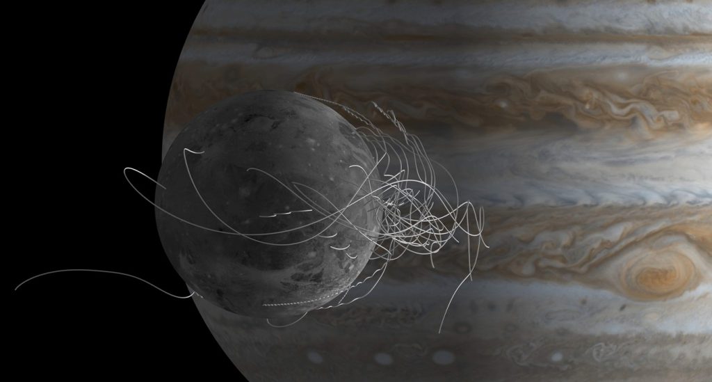
For my PhD project, I modelled the ionosphere of Ganymede, Jupiter's largest moon. The model accounted for several complex cosmic entities: the moon's magnetic field, the exosphere, the relentless solar radiation, and a swarm of Jovian magnetospheric electrons. The model simulates the plasma environment surrounding the moon, capturing the peculiar motion of numerous charged particles. Conveying such an intricate model and grasping how particles move around Ganymede is not easy with static 2-D images and text. For this reason, I created the following animation to explain the model:
The yellow, wiggly lines are solar photons, the steady, blue dots around the moon represent the exosphere, the static, white lines represent magnetic field lines, the red dots are Jovian magnetospheric electrons, and the "dynamic" white lines show the simulated trajectories of Ganymede's ionospheric ions. Importantly, notice the difference in speed between the different types of particles. This was controlled in the animation to match the relative differences in speed of these particles in real life!
"How did you do that!?" is a question I was often asked at conferences. My answer is always: "With MATLAB!". To be more precise, I did it with 'MATLAB only,' relying solely on its core functionalities without the aid of any specialized toolboxes.
In this article, I'll discuss a couple of technical aspects which will help you to effectively create animations involving multiple objects moving at various speeds and temporal resolutions, a quite common scenario in engineering and science. I won't dig into the details of the code behind the animation shown above, but if you're curious about specific aspects of it, then do let me know in the comments!
1. Think in Terms of Frames Instead of Time
In engineering and science we use time to describe the evolution of a certain quantity, but when we create an animation everything should revolve around frames. There are two variables that you need to set when creating an animation: the duration of the animation (in seconds), and the frame rate (fps, frames per second). Let's create a video that lasts 5 seconds and which contains 60 frames per second:
videoDuration = 5;
fps = 60;
Note that the duration of the video is independent of any time-valued entity that you will use in the video, such as the time-dependent coordinates of a moving particle. The video duration and the frames per seconds enable me to calculate the total number of frames in the video:
nFrames = videoDuration * fps
As the director of your own MATLAB animation, it's essential to storyboard your sequence in advance, envisioning the appearance of each frame. For the software developer, the focus shifts from the progression of time 't' in your animation to the specific construction of each frame index. This is because, within MATLAB, movie frames are often crafted within a for-loop, as illustrated in the following code snippet:
for iFrame = 1:nFrames
% update the scene for each frame
end
You might be wondering: how do you synchronize the frame rate and multiple objects that move at varying speeds and temporal resolutions within the simulation? To illustrate this, let's consider an example with two particles. First, load the two timetables containing the time-dependent coordinates for each particle and display the first few rows of both:
load particles.mat
particle1
particle2
Compare the Time variable between the two tables. Notice that the particles start at the same time but move at different speeds and are characterized by different time resolutions.
How do you work your way from time-based coordinates to the frame-based animation? First, you need to identify the simulation timestep dt, or delta time, which represents the simulation time between two consecutive frames. To calculate it, you need the simulation duration tSimEnd, represented in the last movie frame, which differs from the video duration, and the total number of frames. The value of tSimEnd depends on where you want to end the video. In this example, tSimEnd is the last time entry at which the particles' positions were recorded:
tSimEnd = particle1.Time(end); % == particle2.Time(end)
dt = tSimEnd / nFrames
Then, it's just a matter of linearly resampling each timetable using the new calculated timestep and MATLAB's retime function:
particle1 = retime(particle1,'regular','linear','TimeStep',dt)
particle2 = retime(particle2,'regular','linear','TimeStep',dt)
2. Efficiently Manage Graphics Objects
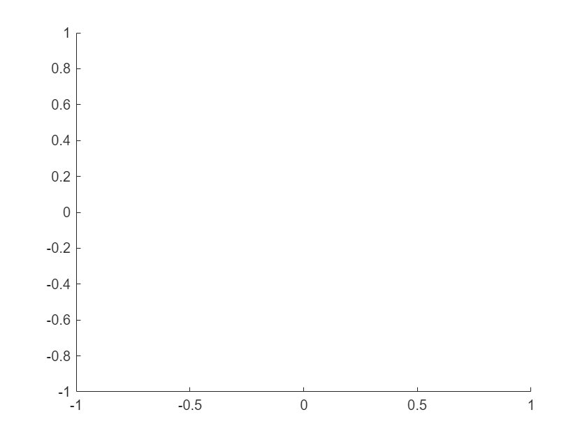
For efficient animations, the less graphics objects you create, the better. We need one axes object to display the motion of both particles, so let's first create the axes object which will host the scene. I know in advance how the particles move; therefore, I can set the axes limits XLim and YLim ahead of time to prevent them from shifting during animation. In addition, the scene will host two particles, so I set the NextPlot property of the axes to "add" to ensure that both particles are displayed:
ax = axes(figure,...
XLim = [-1 1], ...
YLim = [-1 1], ...
NextPlot = "add");
When generating the frames to display the moving particles you might be tempted to approach the problem by destroying and recreating the object on each frame as shown below. I’m using tic toc to measure how long it takes to execute (more on this later):
% !!Example of poor performance!!
tic
for iFrame = 1:nFrames
delete(ax.Children)
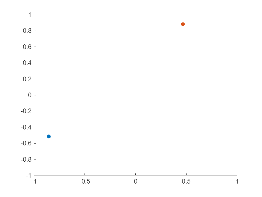
scatter(ax,particle1.x(iFrame),particle1.y(iFrame),'b','filled');
scatter(ax,particle2.x(iFrame),particle2.y(iFrame),'r','filled');
drawnow % refresh screen to show frame
end
The code snippet above plots the updated position of each particle at every frame using two scatter objects. It works, but it is not computationally efficient because at each iteration of the for loop the scatter objects are destroyed and re-created by the graphics system and the plot uses two scatter objects when one could have been used to manage both particles. As a result, it takes a relatively long time to execute (approximately 36 seconds on my machine).
There are two alternatives:
- Initialize only one scatter object and update the XData and YData properties at every iteration;
- Initialize the scatter objects and use matrix transformations.
I am now going to try both approaches. Later, we'll assess the fastest option.
Update XData and YData
First, let's recycle the previously used axes by removing its content:
delete(ax.Children)
In this case, I first initialize the single scatter object defined for two particles and store its handle:
tic
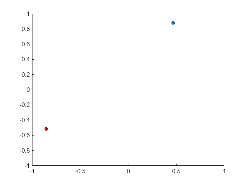
s = scatter(ax, nan(1,2), nan(1,2), [], lines(2), 'filled');
For extra credit, note that I've used the lines function to generate a 2x3 RGB color matrix to define the two scatter points using different colors. There's no need to use real data to initialize a graphics object, so for simplicity I used nan for all values. Then, at every iteration I update the scatter object with the relevant particle coordinates:
for iFrame = 1:nFrames
set(s, ...
XData = [particle1.x(iFrame), particle2.x(iFrame)], ...
YData = [particle1.y(iFrame), particle2.y(iFrame)])
drawnow
end
toc
Notice that tic toc reveals that this approach is quite faster than the previous one, even with only two data points.
Use Matrix Transformations
While it is intuitive to create a scatter point and move its coordinates as time evolves, one can also approach the problem using matrix transformations. You may recall from this great article written by my colleague Ken that with transform objects we can translate, scale, and rotate a set of points which define any object. For this example, I first create an array with two transform objects: one for each particle since they move at different speeds and in different directions.
delete(ax.Children)
tic
h(1) = hgtransform(Parent=ax);
h(2) = hgtransform(Parent=ax);
The transform objects are going to be the parent of the scatter objects, which also need to be initialized. This time, I need to be careful when defining the initial values. In particular, the translation matrix, which is going to operate on the scatter objects, defines the displacement from the initial values. For this reason, it is necessary to initialize the scatter objects with the initial position of the particles rather than using NaNs.
scatter(particle1.x(1),particle1.y(1),'filled',Parent=h(1));
scatter(particle2.x(1),particle2.y(1),'filled',Parent=h(2));
Then, for each iteration I proceed as follows. First, I calculate how much each scatter object needs to be translated from its initial starting position in frame 1 to the new position at the current frame index. Note, we are in the x-y plane, so z is always 0. Then, makehgtform uses those offsets to create the transformation matrix. The first input indicates the type of transformation to be applied (a translation in this case), and the second input contains the translation vector, namely by how much each graphics object will be shifted. Finally, I apply the translation by setting the Matrix property of the transform object h, which is the parent container for the scatter objects. If that takes a moment to settle in, you’re not alone. Transform graphics objects are a unique animal to study in the MATLAB kingdom.
for iFrame = 2:nFrames
% Calculate translation from the position in the first frame
translationVector1 = [particle1.x(iFrame)-particle1.x(1) particle1.y(iFrame)-particle1.y(1) 0];
translationVector2 = [particle2.x(iFrame)-particle2.x(1) particle2.y(iFrame)-particle2.y(1) 0];
% Calculate translation matrix
translationMatrix1 = makehgtform('translate', translationVector1);
translationMatrix2 = makehgtform('translate', translationVector2);
% Apply translation to the scatter objects
h(1).Matrix = translationMatrix1;
h(2).Matrix = translationMatrix2;
drawnow
end
toc
The following table compares the time taken by the three approaches presented above:
|
Approach Type
|
Execution Time (s)
|
|
Re-creating graphics objects
|
36
|
|
Updating scatter plots
|
28
|
|
Using matrix transformations
|
11
|
tic toc times are averages across 5 repetitions (note: these numbers are likely to be different on your machine). Numbers don't lie: in this scenario, transformation matrices provide the fastest approach. By applying a matrix transformation to the scatter data, the position of the rendered points are updated without needing to update the XData, YData, and ZData in the scatter object.
If you need convincing, check the XData and YData properties of the scatter objects after the animation is complete and you’ll find that they retained their initial values. It is not always obvious how one can apply a combination of rotation, scale, and translation matrices, so updating the position properties of the graphics objects remains a valid and often more intuitive alternative.
Do Try This at Home
If you want to try this out on your machine, or get inspiration for your own movie set, then download the source code file movMultiTraj.m for the example presented above:
This version will also show you how to efficiently export the animation to a video file (.avi, .mp4, ...) using the VideoWriter object.
MATLAB enables you to express your creativity in many other ways, for example by operating with the camera (move, rotate, change aperture) or light effects. In this article I limited myself to provide basic steps to get started with animation, but if you're curious to learn about more advanced video effects, then I invite you to download the source code file movSolarSystem.m for the following animation at the bottom of this article:
Enjoy! And why not, feel free to comment below with your ideas on how to create a great movie scene with MATLAB and your science work.


Comments
To leave a comment, please click here to sign in to your MathWorks Account or create a new one.