
Bézier Curves
Bézier Curves and Kronecker's Tensor Product
Last time we talked about Martin Newell's famous teapot. Today we're going to talk about the curves which the teapot is made of. These are known as Bézier curves. These are extremely useful curves, and you'll encounter them in lots of different places in computer graphics.
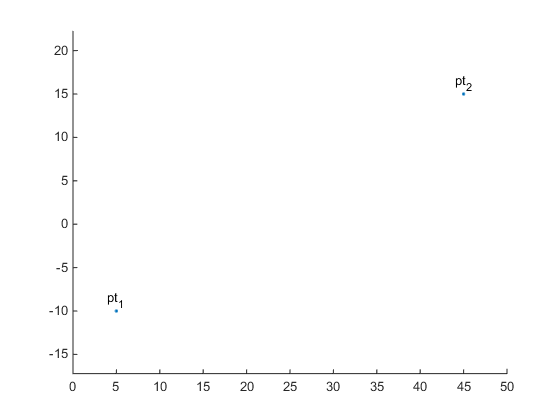
Let's look at how to draw a Bézier curve. We'll start by drawing a line the hard way. We'll start with these two points.
pt1 = [ 5;-10];
pt2 = [45; 15];
We'll use this simple function to label the points.
type placelabel
function placelabel(pt,str)
    x = pt(1);
    y = pt(2);
    h = line(x,y);
    h.Marker = '.';
    h = text(x,y,str);
    h.HorizontalAlignment = 'center';
    h.VerticalAlignment = 'bottom';
And we'll use 'axis equal' to make the scaling uniform in the X & Y directions.
placelabel(pt1,'pt_1');
placelabel(pt2,'pt_2');
xlim([0 50])
axis equal
Now we want to draw the line segment between them. We can think of this line as being a linear combination of the two points.
$$0<=t<=1$$
$$pt(t) = (1-t)*pt_1 + t*pt_2$$
When $t$ is equal to 0, we get:
$$pt(0) = (1-0)*pt_1 + 0*pt_2$$
which is equal to $pt1$. When $t$ is equal to 1, we get:
$$pt(1) = (1-1)*pt_1 + 1*pt_2$$
which is equal to $pt2$. When $t$ is equal to 1/2, we get:
$$pt(1/2) = (1-1/2)*pt_1 + 1/2*pt_2$$
which is the midpoint of the line segment. And indeed, for any value of $t$ between 0 and 1, we get a point on the line.
There are a couple of ways to implement this in MATLAB, but we'll do it the following way. The kron function will give us the Kronecker tensor product of two arrays. This means that it will give us all of the possible products of the elements in those two arrays. So, for example, if we create an array of t values like this:
t = linspace(0,1,101);
We can use kron to multiply all of them by the two coordinate values in each point like this:
pts = kron((1-t),pt1) + kron(t,pt2);
And then we can plot them.
hold on
plot(pts(1,:),pts(2,:))
hold off
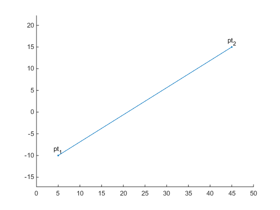
and voila! We have drawn the line between the points.
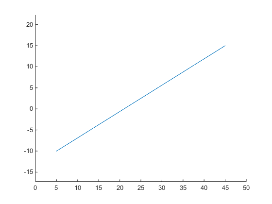
So why do we want to do this? Wouldn't it be easier to just use the line command?
cla
line([pt1(1), pt2(1)],[pt1(2), pt2(2)])
The reason is that we're going to expand this to more points and higher-order functions of $t$. Instead of linear combinations of two points, we're going to create higher-order combinations of three or four points.
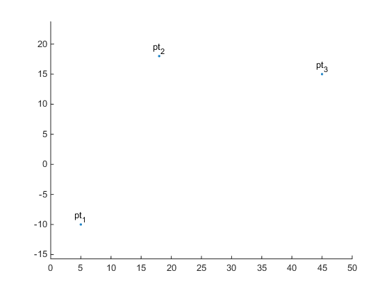
We'll start with the quadratic Bézier curve. This curve takes three points.
pt1 = [ 5;-10];
pt2 = [18; 18];
pt3 = [45; 15];

cla
placelabel(pt1,'pt_1');
placelabel(pt2,'pt_2');
placelabel(pt3,'pt_3');
xlim([0 50])
axis equal
And we've still got $t$ going from 0 to 1, but we'll use second-order polynomials like this:
$$pt(t) = (1-t)^2*pt_1 + 2 (1-t) t*pt_2 + t^2*pt_3$$
These are known as the Bernstein basis polynomials.
We can use the kron function to evaluate them, just as we did in the linear case.
pts = kron((1-t).^2,pt1) + kron(2*(1-t).*t,pt2) + kron(t.^2,pt3);

hold on
plot(pts(1,:),pts(2,:))
hold off
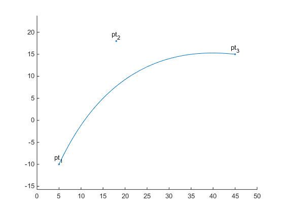
Notice that the resulting curve starts at $pt1$ and ends at $pt3$. In between, it moves towards, but doesn't reach, $pt2$.
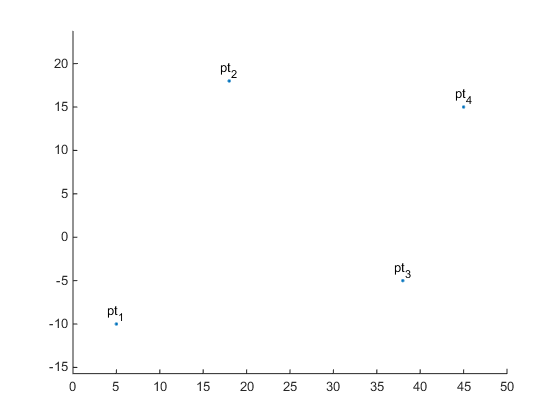
Next we can go up to the cubic Bézier. This is the one which the teapot uses. We'll need 4 points ...
pt1 = [ 5;-10];
pt2 = [18; 18];
pt3 = [38; -5];
pt4 = [45; 15];

cla
placelabel(pt1,'pt_1');
placelabel(pt2,'pt_2');
placelabel(pt3,'pt_3');
placelabel(pt4,'pt_4');
xlim([0 50])
axis equal
... and the following third-order equation:
$$pt(t) = (1-t)^3*pt_1 + 3 (1-t)^2 t*pt_2 + 3 (1-t) t^2*pt_3 + t^3*pt_4$$
pts = kron((1-t).^3,pt1) + kron(3*(1-t).^2.*t,pt2) + kron(3*(1-t).*t.^2,pt3) + kron(t.^3,pt4);

hold on
plot(pts(1,:),pts(2,:))
hold off

Again we can see that the curve starts at the first point and ends at the last point, while moving towards each intermediate point in turn.
Also, notice the pattern of the coefficients of the polynomials in these three examples.
- Order 1 - [1 1]
- Order 2 - [1 2 1]
- Order 3 - [1 3 3 1]
Do you recognize them? They're our old friends the binomial coefficients. You can follow this pattern and create higher order Bézier curves with more points.
So why do computer graphics programmers love Bézier curves? Because they have a lot of useful properties. They're based on those simple polynomials, and we know how to do all sorts of things with polynomials like these.
For example, we can calculate the first derivative with respect to $t$.
a = -3*t.^2 +  6*t - 3;
b =  9*t.^2 - 12*t + 3;
c = -9*t.^2 +  6*t;
d =  3*t.^2;

tvec = kron(a,pt1) + kron(b,pt2) + kron(c,pt3) + kron(d,pt4);
This gives us the tangent vector at any point on the curve. We can add these to our plot with hold on, but we won't draw all of them because it gets too crowded.
for i=1:10:101
    l = line([pts(1,i), pts(1,i)+tvec(1,i)/6], ...
             [pts(2,i), pts(2,i)+tvec(2,i)/6]);
    l.Color = 'green';
end
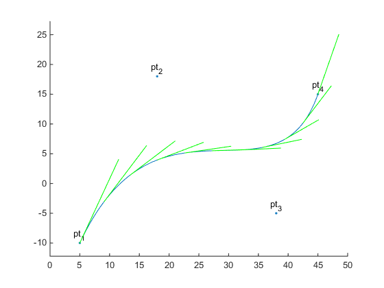
If you look at the values of those derivatives, you'll see an interesting pattern. When $t$ equals 0, the four terms are [-3, 3, 0, 0]. That means that the tangent of the start of the curve is simply $3pt_2 - 3pt_1$. The same thing happens at the other end when $t$ equals 1.
This makes it easy to connect two Bézier curves so that they are tangent at the meeting point. You just make the last two points of the first curve colinear with the first two points of the second curve.
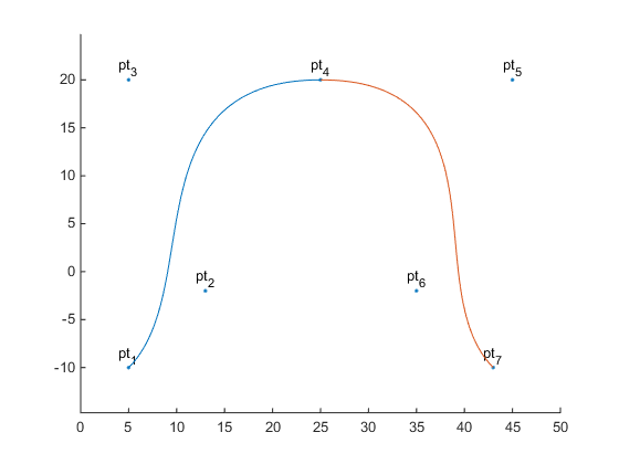
cla
xlim([0 50])
axis equal

pt1 = [ 5;-10];
pt2 = [13; -2];
pt3 = [ 5; 20];
pt4 = [25; 20];

placelabel(pt1,'pt_1');
placelabel(pt2,'pt_2');
placelabel(pt3,'pt_3');
placelabel(pt4,'pt_4');

pt5 = [45; 20];
pt6 = [35; -2];
pt7 = [43;-10];

placelabel(pt5,'pt_5');
placelabel(pt6,'pt_6');
placelabel(pt7,'pt_7');
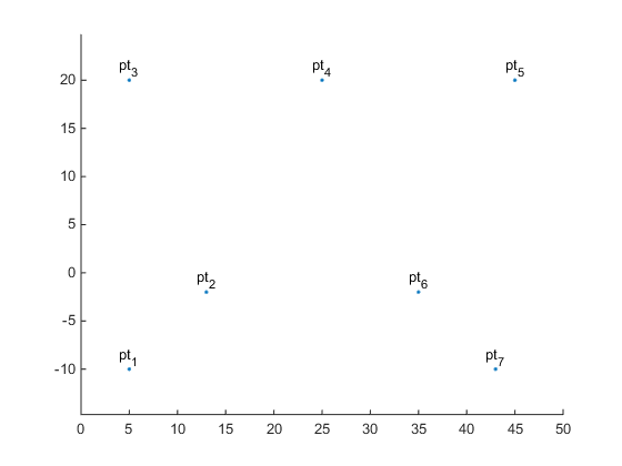
Notice that $pt3$, $pt4$, and $pt5$ are colinear:
pt4 - pt3
pt5 - pt4
ans =

    20
     0


ans =

    20
     0
And if we plot the curves, we can see that we get a nice, smooth join where they meet.
pts1 = kron((1-t).^3,pt1) + kron(3*(1-t).^2.*t,pt2) + kron(3*(1-t).*t.^2,pt3) + kron(t.^3,pt4);
pts2 = kron((1-t).^3,pt4) + kron(3*(1-t).^2.*t,pt5) + kron(3*(1-t).*t.^2,pt6) + kron(t.^3,pt7);

hold on
plot(pts1(1,:),pts1(2,:))
plot(pts2(1,:),pts2(2,:))
hold off
You can find a list of other useful properties of the Bézier curve at this Wikipedia page.
The teapot is actually made of Bézier patches. These are parametric surfaces which are made from the same math as Bézier curves, but with two parameters (usually called $u$ and $v$) instead of the one parameter (i.e. $t$) that we've been using here. We'll come back to investigate Bézier patches in a future post, but first we're going to explore how to draw some other useful curves.
- 类别:
- Geometry

