State Taxes

If you live in the US, you probably filed your taxes sometime in the last couple of months. If you're like me, that got you looking at data about taxes. One nice source of tax data is the US Census Bureau.

Justice Louis Brandeis called the states the laboratories of democracy. They're also the laboratories of tax policy. If we go to this page of the census bureau's site, we can get a lot of details about how different types of taxes contribute to the various states' revenues.

The first step is to hit the download button on that page. That will give us two files named 'STC_2014_STC005_with_ann.csv' and 'STC_2014_STC005_metadata.csv'. The first contains all of the tax data. The second contains the names of the different types of taxes.

MATLAB's readtable command sucks that in pretty easily, although it warns about things like spaces and quotes in the names of the taxes.

t = readtable('STC_2014_STC005_with_ann.csv','Delimiter',',','HeaderLines',1);
m = readtable('STC_2014_STC005_metadata.csv');

Warning: Variable names were modified to make them valid MATLAB identifiers. 
Warning: Variable names were modified to make them valid MATLAB identifiers. 

There are a couple of different types of information in the data file.

The 3rd column contains the names of the states.

state_names = table2array(t(2:end,3));
state_names(1:5)

ans = 

    'Alabama'
    'Alaska'
    'Arizona'
    'Arkansas'
    'California'

The 4th column contains the total amount each state took in for 2014.

state_totals = table2array(t(2:end,4));
state_totals(1:5)

ans =

     9293754
     3392869
    13084043
     8936781
   138069870

And the rest of the table contains the revenues for each type of tax for each state.

raw_tax_receipts = table2array(t(2:end,5:end));
raw_tax_receipts(1:5,1:5)

ans =

      329598     4812674     2393192     2419482      181427
      128076      257696           0      257696       39078
      823508     7759625     5994048     1765577       71136
     1077377     4324157     3130274     1193883       51618
     2176236    50002053    37224077    12777976      354297

And we'll need the tax names which are in the 2nd column of the metadata starting at row 4.

raw_tax_names = m.Id(4:end);

But the different types of taxes aren't a flat list. Some of them are "roll-ups" of the others. For example, the tax named "Income Taxes" (column 23) is the sum of the two taxes named "Individual Income Taxes" and "Corporation Net Income Taxes" (columns 24 and 25). This means that we need to break them into two sets. First we'll look at the top level groups.

top_level = [1 2 13 23 26];
tax_receipts = raw_tax_receipts(:,top_level);
tax_names = raw_tax_names(top_level);

Next we need to decide how we're going to visualize this data. One challenge is that the total tax revenues of the various states vary pretty widely. California took in 138 million dollars, but South Dakota only took in 1.6 million dollars. To compare them, it will help to normalize our data.

This is actually a good job for something called a "stacked percentage column chart". MATLAB doesn't have one built in, because it isn't actually useful for a lot of things we do, but it is pretty easy to create one with the bar command. All we need to do is multiply the various tax revenues of the different states by 100 divided by the total tax revenues for that state. We'll also want the names of the states along the X axis. The result is a function that looks something like this:

function h = normbar(data,totals,rownames)
  scale = 100./repmat(totals,[1 size(data,2)]);
  h = bar(data.*scale,'stacked','BarWidth',1);
  ax = gca;
  ax.Position=[.05 .235 .93 .72];
  axis(ax,'tight')
  ax.XTick = 1:50;
  ax.XTickLabel = rownames;
  ax.XTickLabelRotation = 90;

h = normbar(tax_receipts, state_totals, state_names);

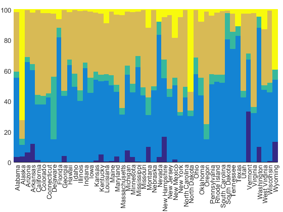
But that's really hard to understand without a legend. One problem with stacked bar charts is that they stack from the bottom up, but the legend goes from the top down. To fix that, we'll need to use fliplr.

for i=1:length(h)
    h(i).DisplayName = tax_names{i};
end
legend(fliplr(h),'Location','northoutside')

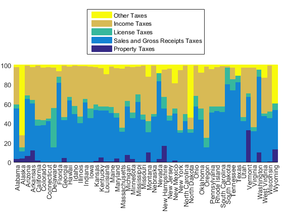
That helps a little bit. We can now start to see some differences between the states. For example, we can see that Vermont depends a lot on property taxes.

But it's hard to compare the different states when they're in alphabetical order. It'd be better to rank them by a particular type of tax revenue. For example, if we sort them by property tax, we'll get Vermont on the right, along with other states which are dependent on property taxes.

tax_index = 1;
[~,idx] = sort(tax_receipts(:,tax_index)./state_totals);
normbar(tax_receipts(idx,:), state_totals(idx), state_names(idx));
title(['States ranked by "', tax_names{tax_index}, '"'])

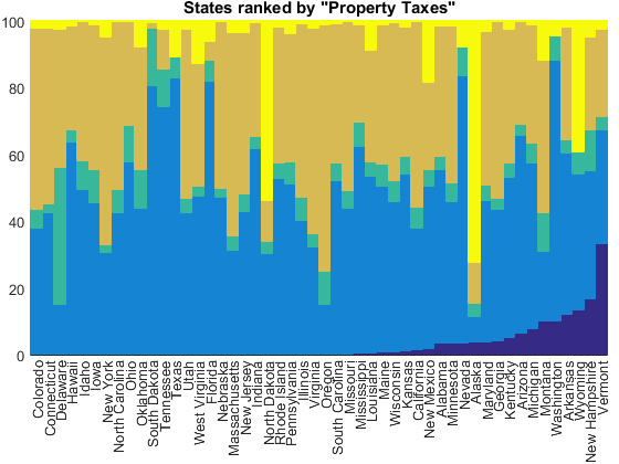
But if we sort by income taxes, we'll get Oregon on the right and the states with no income taxes on the left.

tax_index = 4;
[~,idx] = sort(tax_receipts(:,tax_index)./state_totals);
normbar(tax_receipts(idx,:), state_totals(idx), state_names(idx));
title(['States ranked by "', tax_names{tax_index}, '"'])

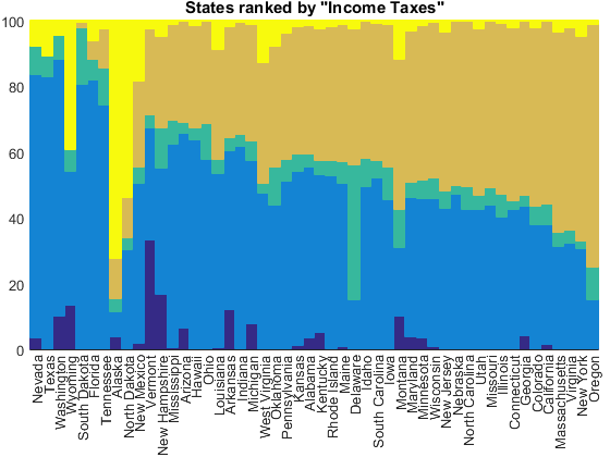
The category labeled "Other Taxes" looks kind of interesting, but it's kind of hard to guess what it means from the name. It's made up of a collection of unrelated taxes.

tax_index = 5;
[~,idx] = sort(tax_receipts(:,tax_index)./state_totals);
normbar(tax_receipts(idx,:), state_totals(idx), state_names(idx));
title(['States ranked by "', tax_names{tax_index}, '"'])

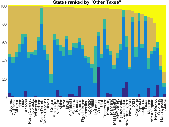
To see what's going on here, we need to drill down to those subcategories that I mentioned earlier.

other_taxes = 27:30;
other_tax_receipts = raw_tax_receipts(:,other_taxes);
other_totals = raw_tax_receipts(:,26);
other_tax_names = raw_tax_names(other_taxes);

h = normbar(other_tax_receipts, other_totals, state_names);

for i=1:length(h)
    h(i).DisplayName = other_tax_names{i};
end
legend(fliplr(h),'Location','northoutside');

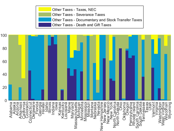
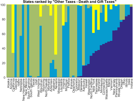
We see three important taxes hiding in this group. First is called "death and gift taxes" which are apparently important in Indiana.

tax_index = 1;
[~,idx] = sort(other_tax_receipts(:,tax_index)./other_totals);
normbar(other_tax_receipts(idx,:), other_totals(idx), state_names(idx));
title(['States ranked by "', other_tax_names{tax_index}, '"'])

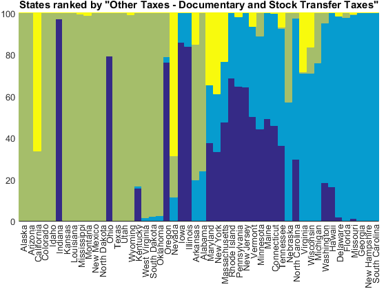
Next is "documentary and stock transfer taxes" which are apparently important in Georgia, New Hampshire, and South Carolina.

tax_index = 2;
[~,idx] = sort(other_tax_receipts(:,tax_index)./other_totals);
normbar(other_tax_receipts(idx,:), other_totals(idx), state_names(idx));
title(['States ranked by "', other_tax_names{tax_index}, '"'])

And finally, there's something called a "severance tax". Can you guess what this is from the names of the states which depend a lot on it?

tax_index = 3;
[~,idx] = sort(other_tax_receipts(:,tax_index)./other_totals);
normbar(other_tax_receipts(idx,:), other_totals(idx), state_names(idx));
title(['States ranked by "', other_tax_names{tax_index}, '"'])

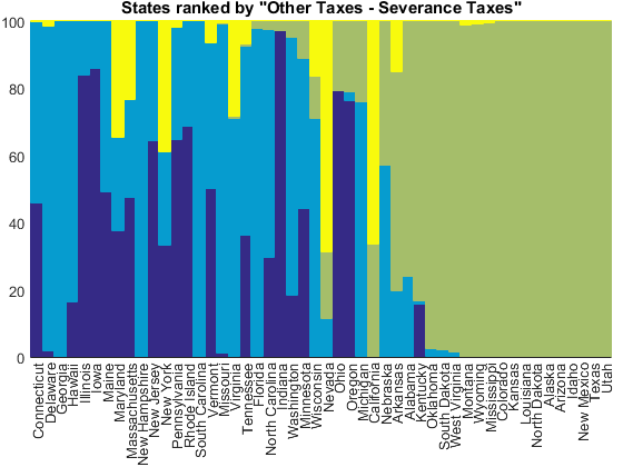
That's right, a severance tax is the money that a company pays to the state when it extracts a non-renewable resource such as oil, coal, or natural gas.

But those last three charts were normalized to the size of the "Other Taxes" category. That's actually a small factor for most of these states, so let's go back and normalize against the state totals again.

[~,idx] = sort(other_tax_receipts(:,tax_index)./state_totals);
h = normbar(other_tax_receipts(idx,:), state_totals(idx), state_names(idx));

for i=1:length(h)
    h(i).DisplayName = other_tax_names{i};
end
legend(fliplr(h),'Location','northoutside');

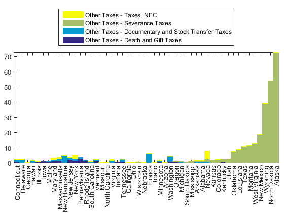
Now we can see that the states which show up with large revenues from "Other" are the ones that depend a lot on these severance taxes. They're the states which take in a lot of payments for the extraction of natural resources, such as Alaska's famous oil and gas revenues.

What interesting patterns can you find in this dataset? Can you use some of these techniques for other types of data?

Get the MATLAB code

Published with MATLAB® R2015a