
Homogeneous Coordinates
Homogeneous Coordinates
In my recent posts about tiling polygons (link1, link2), you might have noticed that I used a rather unusual representation for my coordinates.
Instead of having a vector of X coordinates and a vector of Y coordinates, I had a 3xN array of values that looked something like this:
pts = [4  4 -1 -1  2  2  1  1  0  0  3  3; ...
       1  3  3 -1 -1  1  1  0  0  2  2  1; ...
       1  1  1  1  1  1  1  1  1  1  1  1];
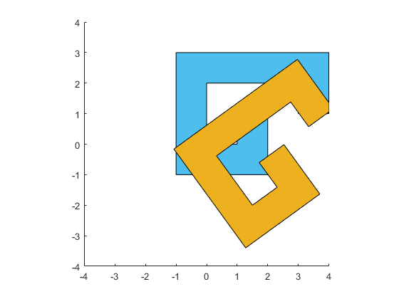
Let's start by drawing the polygon I defined in that pts array. We can do that like so:
axis equal
xlim([-4 4])
ylim([-4 4])
h1 = patch('FaceColor',[0.3010 0.7450 0.9330]);
h1.XData = pts(1,:) ./ pts(3,:);
h1.YData = pts(2,:) ./ pts(3,:);
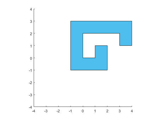
But why did I use that odd 3x12 representation, and what does the row of 1's represent? This representation is called homogeneous coordinates. They've been around for almost 200 years, but they were kind of an obscure curiosity until computer graphics programmers started using them. We use them constantly in computer graphics, and they're the fundamental representation in the rendering library which underlies MATLAB's new graphics system. Let's take a look at how homogeneous coordinates work, and why computer graphics programmers love them so much.
Notice that when I turned the first row of the array into the XData of the patch, I divided by the third row. I did the same thing when I turned the second row into the YData. I actually skipped this step in the tiling posts to keep things simple, but this is how we move from the projective space of homogeneous coordinates into the Euclidean space we're familiar with. Every 2D Euclidean point is equivilent to an infinite set of homogeneous points in the projective space. These points lie on a line which goes through a point at infinity.
In other words, all of these 3D homogeneous points
- [6 3 1]
- [12 6 2]
- [3 1.5 .5]
- [.6 .3 .1]
- [60 30 10]
are equivilent to the same point in 2D Euclidean space (i.e. [6 3]).
OK, that's kind of interesting, but why do computer graphics programmers like homogeneous coordinates so much? The answer is that in computer graphics we spend a lot of our time computing transformations between coordinate systems, and that becomes much simpler in homogeneous coordinates.
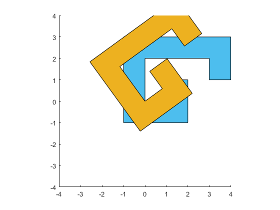
So to understand why we like this unusual representation so much, we're going to need to look at some transformations. Let's start with a simple one that you probably learned at some point. We're going to rotate that polygon around the origin by an angle of pi/5. To do that, we create a matrix that looks like this:
mrot = [cos(pi/5), -sin(pi/5), 0; ...
        sin(pi/5),  cos(pi/5), 0; ...
                0,          0, 1];
And we can multiply it by our points to create a new set of points.
p2 = mrot*pts;
And if we draw them the same way we did our earlier points, then we get a rotated version of the polygon.
x = p2(1,:) ./ p2(3,:);
y = p2(2,:) ./ p2(3,:);
h2 = patch('FaceColor',[0.9290 0.6940 0.1250]);
h2.XData = x;
h2.YData = y;

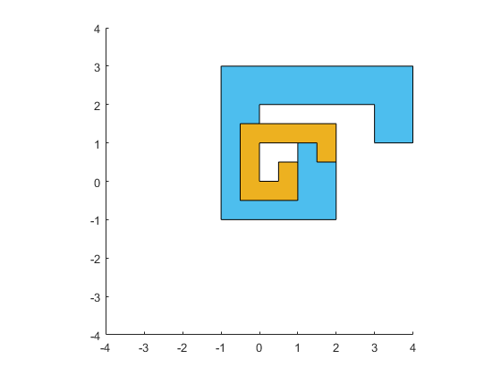
In the same way, we can scale the polygon around the origin by creating a matrix with the scale factors in locations (1,1) and (2,2).
mscal = [1/2   0 0; ...
           0 1/2 0; ...
           0   0 1];
p2 = mscal*pts;
h2.XData = p2(1,:) ./ p2(3,:);
h2.YData = p2(2,:) ./ p2(3,:);
And a reflection around the Y=0 line just involves changing the sign of one of the diagonal elements:
mrefl = [1  0 0; ...
         0 -1 0; ...
         0  0 1];
p2 = mrefl*pts;
h2.XData = p2(1,:) ./ p2(3,:);
h2.YData = p2(2,:) ./ p2(3,:);
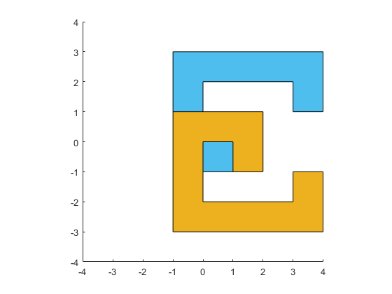
But that really doesn't answer the question. We could have done the same thing with a 2x2 transform matrix and a 2xN array of points. Things get a little more interesting if we look at translations. We can't fit a translation into the 2x2 matrix, but we can fit it into the third column of our 3x3. And then we can translate objects using the same mechanism we're using for rotating and scaling.
mxlat = [1 0  1.5; ...
         0 1 -2; ...
         0 0  1];
p2 = mxlat*pts;

h2.XData = p2(1,:) ./ p2(3,:);
h2.YData = p2(2,:) ./ p2(3,:);
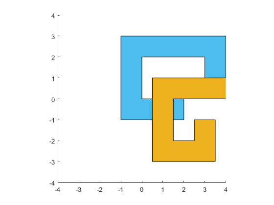
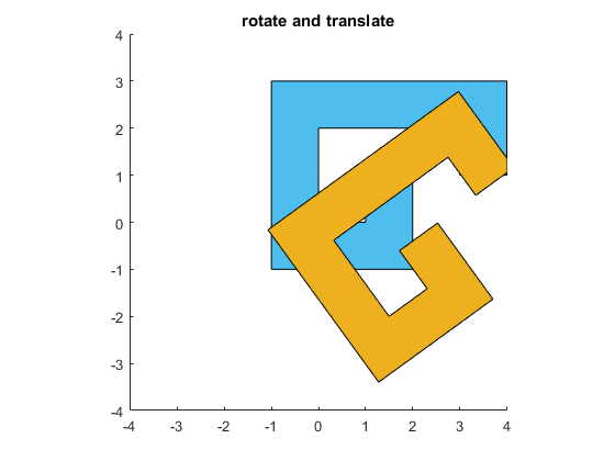
But even that's not too compelling. You can deal with translations without having a third row if you use a 2x3 transform matrix. The problem with that is that these 2x3 matrices aren't as easy to combine as our 3x3 matrices are. For example, we can perform a rotation and a translation by simply multiplying the two matrices we've already created.
p2 = mxlat*mrot*pts;
h2.XData = p2(1,:) ./ p2(3,:);
h2.YData = p2(2,:) ./ p2(3,:);
title('rotate and translate')
That's nice and simple, but computer graphics programmers didn't really fall in love with homogeneous coordinates until we started drawing things in perspective.
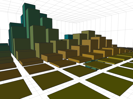
Perspective projections allow us to create realistic looking scenes where distant objects appear smaller than near objects, like this:
figure
bar3(peaks(15))
ax = gca;
ax.Projection='perspective';
ax.CameraViewAngle = 50;
ax.CameraPosition=[16 14 2];
ax.CameraTarget = [7 7 0];
light('Position',[6 -5 8])
But perspective projections are challenging to represent in Euclidean space. In the world of homogeneous coordinates, perspective projections are quite natural. They're what we get when we put values in the bottom row of the transformation matrix.
Back in our 2D world, if we want to make the top of our polygon recede into the distance, we just need to add a non-zero element at (3,2) in our matrix. This will make the W coordinate of the output a function of the Y coordinate of the input. When we do that, the division by W will scale down the top of the scene and scale up the bottom of the scene.
close
mproj = [1   0 0; ...
         0   1 0; ...
         0 1/3 1];
p2 = mproj*pts;
h2.XData = p2(1,:) ./ p2(3,:);
h2.YData = p2(2,:) ./ p2(3,:);
title('projection')
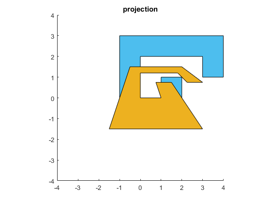
This gives us the effect of receding into the distance that we need for a perspective projection. Now we are ready to start drawing in a "galaxy far, far away".
Of course MATLAB's graphics system isn't 2D only. It supports 3D. Because of this, it actually uses homogeneous coordinates with 4 values rather than the 3 values we've used so far. These 4 values are called X, Y, Z, and W. So I could recreate my polygon (which is at Z==0) like this:
clf
pts = [4  4 -1 -1  2  2  1  1  0  0  3  3; ...
       1  3  3 -1 -1  1  1  0  0  2  2  1; ...
       0  0  0  0  0  0  0  0  0  0  0  0; ...
       1  1  1  1  1  1  1  1  1  1  1  1];
axis equal
xlim([-4 4])
ylim([-4 4])
h1 = patch('FaceColor',[0.3010 0.7450 0.9330]);
h1.XData = pts(1,:) ./ pts(4,:);
h1.YData = pts(2,:) ./ pts(4,:);
h1.ZData = pts(3,:) ./ pts(4,:);

And our transforms become 4x4 matrices. MATLAB comes with a handy function named makehgtform which will create these matrices. For example, I can create the 4x4 version of that rotation matrix like so:
mrot = makehgtform('zrotate',pi/5)
mrot =

    0.8090   -0.5878         0         0
    0.5878    0.8090         0         0
         0         0    1.0000         0
         0         0         0    1.0000
And we can use that just like we did earlier.
p2 = mrot*pts;

h2 = patch('FaceColor',[0.9290 0.6940 0.1250]);
h2.XData = p2(1,:) ./ p2(4,:);
h2.YData = p2(2,:) ./ p2(4,:);
h2.ZData = p2(3,:) ./ p2(4,:);

Or we can use the hgtransform object to perform the transformation. This object has a property named Matrix. That takes one of these 4x4 matrices and applies it to every object which is "parented" to the hgtransform. This is often the most efficient way to transform a graphics object because the transformation is actually done by the graphics card.
delete(h2)
g = hgtransform;
g.Matrix = mrot;
h2 = patch('FaceColor',[0.9290 0.6940 0.1250],'Parent',g);
h2.XData = pts(1,:);
h2.YData = pts(2,:);
h2.ZData = pts(3,:);
The makehgtform command has options for most of the common transformations, as well as more complex ones such as rotating around an arbitrary axis. It will even let you list several transformations and then return the matrix which would result if you multiplied them together as we did above. So we can recreate the combination of translate and rotate we did earlier with this single call.
g.Matrix = makehgtform('translate',[1.5 -2 0], 'zrotate',pi/5);
So does this mean that we can use hgtransform to apply things like that cool perspective effect?
Well, no ...
mproj = [1   0 0 0; ...
         0   1 0 0; ...
         0   0 1 0; ...
         0 1/3 0 1];
try
    g.Matrix = mproj;
catch me
    disp(me.message)
end
Invalid value for Matrix property
The reason is that even though the entire graphics pipeline is implemented using homogeneous coordinates, there are actually 3 types of transform matrices in the pipeline. We call these model, view, and projection matrices. The hgtransform object is controlling the model transform. The view transform is controlled by the properties CameraPosition, CameraTarget, and CameraUpVector on the axes. And the projection matrix is controlled by the properties CameraViewAngle and Projection on the axes.
There are restrictions on what types of matrices are allowed in each of these three transforms. This is because the code that runs on the GPU at the different stages of the graphics pipeline makes assumptions about its input to maximize performance. Currently the model transform does not allow reflections or perspective transformations.
But we can do these types of transformations using the technique we were using at the beginning of this post. The difference is that in this case MATLAB is doing all the computation on the CPU instead of the GPU. This will generally mean that the performance will not be as good as it would be if we used hgtransform to perform the transformation on the GPU, but it does give us access to the transformations which hgtransform doesn't support.
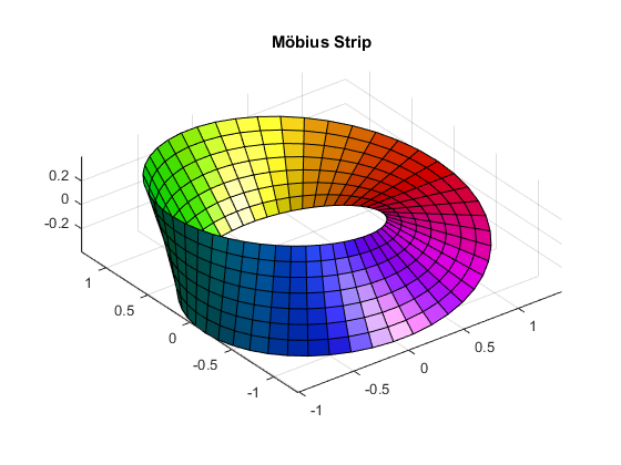
I hope that gave you an idea of why computer graphics programmers love this odd representation for their coordinates. Perhaps you'd like to learn more about this and about some of the many other interesting discoveries of August Ferdinand Möbius, the man who first introduced the world to homogeneous coordinates.
[u,v] = meshgrid(linspace(0,2*pi,50),linspace(-.4,.4,8));
surf(cos(u)+v.*cos(u/2).*cos(u),sin(u)+v.*cos(u/2).*sin(u),v.*sin(u/2),u)
axis equal
camlight
colormap(hsv)
title('Möbius Strip')
- カテゴリ:
- Rendering

