
Which MATLAB Optimization functions can solve my problem?
The solvers function from Optimization toolbox is one of my favourite enhancements of R2022b because it helps improve my knowledge of which algorithms can solve my problems.
Solving Rosenbrock with the default algorithm
$ f(x)=100\left ( x_2 - x_1^2\right )^2 + (1-x_1)^2 $
The minimum is at (1,1) which is inside a long, narrow and flat valley. Many Optimization solvers find the valley rather easily but struggle with finding the global mimimum within it.
rosen = @(x,y) 100*(y - x.^2).^2 + (1 - x).^2;
fcontour(rosen,[-0.5,2.0],LevelStep=10)
hold on
scatter(1,1,300,'r.');
hold off
title("Contour plot of Rosenbrock's function. Global minimum shown in red")

% Set up a couple of Optimization variables and apply boundaries
x = optimvar("x",LowerBound=-3,UpperBound=3);
y = optimvar("y",LowerBound = 0,UpperBound=9);
%Define the objective function
obj = 100*(y - x^2)^2 + (1 - x)^2;
%Set up the Optimization problem
prob = optimproblem(Objective=obj);
%choose a starting guess
x0.x = -2.1;
x0.y = 2.2;
% solve the problem
[sol,fval,exitflag,solution] = solve(prob,x0)
MATLAB analysed the problem and decided to use lsqnonlin as the solver. This turned out rather well for us as it went on to find the minimum without any difficulty. There were only 27 function evaluations.
What other algorithms could solve this problem?
You might ask yourself, however, out of all of the Optimization solvers in both Optimization Toolbox and Global Optimization Toolbox, which of them are capable of solving this problem as well? This is what the solvers function does for us. Give it an Optimization problem and it will return the default solver that MATLAB would choose for that problem.
[autosolver,allsolvers] = solvers(prob);
fprintf("The default solver for this problem is %s\n",autosolver)
It also returns all other solvers that could tackle the input problem.
allsolvers'
[sol,fval,exitflag,solution] = solve(prob,x0,Solver="fmincon")
So fmincon can and did solve the problem but it had to work much harder with 71 function evaluations. Just because the solvers function determines that an algorithm is capable of tackling a problem doesn't necessarily mean its a good fit. An example of a really bad fit for this problem is Simulated Annealing.
[sol,fval,exitflag,solution]= solve(prob,x0,Solver="simulannealbnd")
Yikes! That's rather far from the actual solution and we've already burned though over a thousand function evaluations. Perhaps simulated annealing isn't such a good idea for this function after all.
Let's try every solver that's valid for this problem using default settings for each one
variableNames = ["x solution","y solution","objective value","function evaluations"];
results = array2table(NaN(numel(allsolvers), numel(variableNames)));
results.Properties.VariableNames = variableNames;
results.Properties.RowNames = allsolvers;
for solverNum = 1:numel(allsolvers)
solver = allsolvers(solverNum);
% I want each solver to be quiet while it works.
options=optimoptions(solver,Display="None");
if solver=="surrogateopt"
options=optimoptions(options,PlotFcn=[]);
end
[sol,fval,exitflag,solution] = solve(prob,x0,Solver=solver,Options=options);
%Some solvers have solution.funcCount, others have solution.funccount
if isfield(solution,'funcCount')
funcount = solution.funcCount;
else
funcount = solution.funccount;
end
results.("x solution")(solverNum) = sol.x;
results.("y solution")(solverNum) = sol.y;
results.("objective value")(solverNum) = fval;
results.("function evaluations")(solverNum) = funcount;
end
results
It seems that MATLAB's default choice for this problem, lsqnonlin, was a good one. Indeed it was the best one. That's not always the case though.
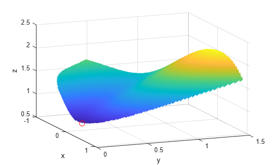
Which algorithm is best for Rastigrin's function?
Consider Rastigrin's function. This is another classic test function in numerical optimization with many local minima and a global minimum at (0,0):
ras = @(x, y) 20 + x.^2 + y.^2 - 10*(cos(2*pi*x) + cos(2*pi*y));
Plotting it shows just how many local minima there are
fsurf(ras,[-3 3],"ShowContours","on")
title("rastriginsfcn(x,y)")
xlabel("x")
ylabel("y")

Usually you don't know the location of the global minimum of your objective function. To show how the solvers look for a global solution, this example starts all the solvers around the point [2,3], which is far from the global minimum. It also uses finite bounds of -70 to 130 for each variable
x = optimvar("x","LowerBound",-70,"UpperBound",130);
y = optimvar("y","LowerBound",-70,"UpperBound",130);
prob = optimproblem("Objective",ras(x,y));
x0.x = 2;
x0.y = 3;
solve(prob,x0)
[autosolver,allsolvers] = solvers(prob)
Sweeping across all valid solvers again and we see that, this time, global Optimization functions such as patternsearch, particle swarm and simulated annealing do much better.
variableNames = ["x","y","objective value","function evaluations"];
results = array2table(NaN(numel(allsolvers), numel(variableNames)));
results.Properties.VariableNames = variableNames;
results.Properties.RowNames = allsolvers;
for solverNum = 1:numel(allsolvers)
solver = allsolvers(solverNum);
% I want each solver to be quiet while it works.
options=optimoptions(solver,Display="None");
if solver=="surrogateopt"
options=optimoptions(options,PlotFcn=[]);
end
[sol,fval,exitflag,solution] = solve(prob,x0,Solver=solver,Options=options);
%Some solvers have solution.funcCount, others have solution.funccount
if isfield(solution,'funcCount')
funcount = solution.funcCount;
else
funcount = solution.funccount;
end
results.("x")(solverNum) = sol.x;
results.("y")(solverNum) = sol.y;
results.("objective value")(solverNum) = fval;
results.("function evaluations")(solverNum) = funcount;
end
results
It's worth bearing in mind that these 'solver sweeps' only consider the default settings for each solver. Each solver has a range of options that can improve performance and solution quality that haven't been considered here but we have made a good start in exploring the algorithms we can bring to bear on our problem.
To learn more about the Optimization algorithms available in MATLAB, take a look at the documentation.


评论
要发表评论,请点击 此处 登录到您的 MathWorks 帐户或创建一个新帐户。