Pi day: Using AI, GPUs and Quantum computing to compute pi
14th March is Pi Day, celebrated by geeks everywhere and a great excuse for technical computing bloggers to publish something tenuously related to pi and their favorite technology of choice. This is not the first pi day celebration on a MathWorks blog and it will not be the last. Here are some of our past takes on the subject
- 2023 Adam Danz celebrated pi day with a pi patch
- 2018 Cleve Moler Looked at the first 10,000 digits of pi
- 2015 Loren Shure asked The Ultimate Pi Day is Over...Now What?
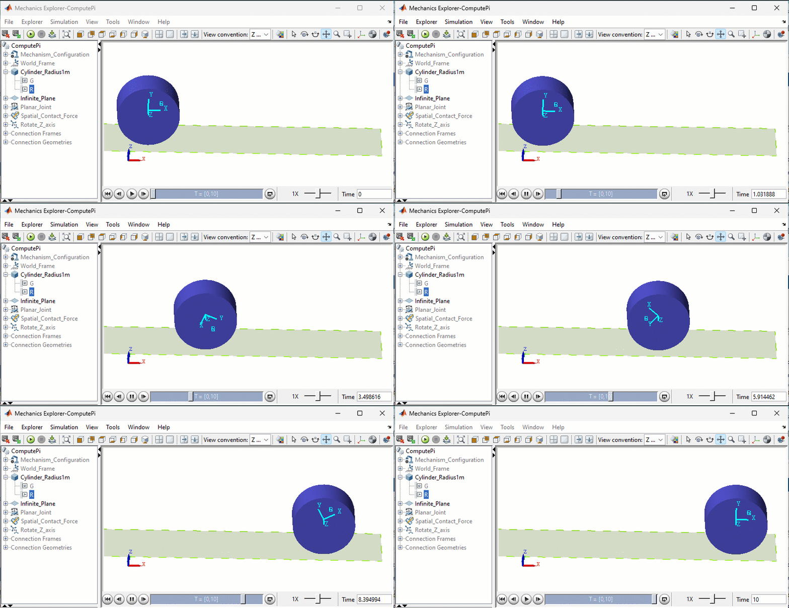
This year, over at The Simulink Blog, Guy has been using Simscape Multibody to simulate one way our ancestors could have computed pi -- by rolling a big stone cylinder down a hill.

I, on the other hand, will be at the other end of the time line by making use of Artificial Intelligence, GPUs and Quantum computing. If only I could have fitted in 'Blockchain', I would have won buzzword bingo!
Using AI to compute pi
One method for computing pi uses a Monte Carlo simulation. Its so well known that it's actually used as a demonstration of what a Monte Carlo method is in the wikipedia entry for Monte Carlo Method! For the sake of brevity, I'll leave you to explore the mathematics for yourself. Today, I'm just going to go ahead and use The MATLAB AI Chat Playground and ask it how to code such a simulation in MATLAB.

This is what it came up with, with a small modification by me to show more decimal points:
%Added by Mike to show more decimal points in the result
format long
% Number of random points to generate
numPoints = 1e6;
% Generate random points in the range [0,1]
x = rand(numPoints, 1);
y = rand(numPoints, 1);
% Count the number of points inside the unit circle
insideCircle = (x.^2 + y.^2) <= 1;
% Estimate pi using the ratio of points inside the circle to total points
piEstimate = 4 * sum(insideCircle) / numPoints
One of the issues with Monte Carlo simulations is that they require a huge number of samples to get an accurate answer. Indeed, the 1 million samples suggested by the AI only gives us 1 or 2 correct decimal places for pi. For more accuracy, you need a lot more samples. Not just a few million more but millions of millions more.
On my machine, the above code completes in a fraction of a second: 0.014 seconds to be precise which works out at around 71.4 million samples a second. Sounds pretty fast but it would take almost 4 hours to compute 10^12 samples and, as written, I'd run out of memory if I even tried it.
Starting from the above code and using various parallelisation and optimisation methods, I got close to 700 million samples a second on my 8 core machine and might even be able to squeeze out some more but I'll save that discussion for another time. Today, I'll take another route.
Computing pi on the GPU
Without GPUs, many of the machine learning techniques we use today would not be computationally feasible and technologies like the AI Chat Playground would not exist. I thought it would be fitting, therefore, to show how you'd accelerate the above AI-generated monte carlo code using the very devices that power modern AI.
It often surprises me that many people don't know how extensive the GPU support is in MATLAB. Using Parallel Computing Toolbox, over 1,000 MATLAB functions 'just work' on a GPU when you supply them with a gpuArray. Not only that but MATLAB can automatically compile a subset of the language to run on the GPU using arrayfun. You can even get MATLAB to write CUDA code using GPU Coder.
Today, however, let's keep it simple. Here's the code from AI Chat Playground, modified to run on my NVIDIA GPU and with 100 million samples instead of only 1 million. Other than changing the numPoints line, I only needed to modify the two calls to rand to request that the random numbers, x and y are generated on the GPU. All subsequent computations automatically work on the GPU. More details on how this works in my post How to make a GPU version of this MATLAB program by changing two lines
% This code needs an NVIDIA GPU and Parallel Computing Toolbox
% Number of random points to generate
numPoints = 1e8;
% Generate random points in the range [0,1]
x = rand(numPoints, 1, "gpuArray");
y = rand(numPoints, 1, "gpuArray");
% Count the number of points inside the unit circle
insideCircle = (x.^2 + y.^2) <= 1;
% Estimate pi using the ratio of points inside the circle to total points
piEstimate = 4 * sum(insideCircle) / numPoints
Timing this correctly (A simple tic/toc isn't the way to go with GPU computations, see Measure and Improve GPU Performance for details) resulted in a speed of 0.06 seconds which gives us 1,666 million samples per second. That's a very nice speed up for very little work.
I can't push the above code much further though since I quickly run out of memory on the GPU. One way to proceed is to split the simulation into chunks. I'm also going to use single precision since its faster on my GPU, uses less memory and the drop in precision isn't an issue here. Let's also put the code into a function
function pi = piMonteCarloSplit(N,numChunks)
count = 0;
for i =1:numChunks
x = rand(N/numChunks, 1, "single", "gpuArray");
y = rand(N/numChunks, 1, "single", "gpuArray");
count = count + sum((x.^2 + y.^2)<1);
end
pi = 4*count/N;
end
Time this using 100x more samples than before: 1e10 split into 100 chunks, using a timing technique described at Measure and Improve GPU Performance
dev = gpuDevice();
wait(dev);
tic
piEstimate = piMonteCarloSplit(1e10,100);
wait(dev);
toc
10,000 million samples in 3.123 seconds gives 12,195 million samples per second. Hugely faster than where we started with barely any additional effort at all. Here's the estimate for pi we get now
piEstimate
Even with 10,000 million samples, I only got 4 decimal places correct. There's a reason why this technique is not used if high precision for computing pi is what you need.
Using additional techniques, I eventually squeezed almost 17,000 million samples a second out of my GPU and there could be more performance on the table. I may write this up another time if there is sufficient interest. The point here is that it can be really easy to get started with porting a lot of MATLAB code to the GPU and the performance is pretty good!
For reference, my GPU is an NVIDIA GeForce RTX 3070 and I'm also using it as the display driver.
Calculating pi using a quantum computer
Guy's post took us back to ancient times. I wanted to take a glimpse at the future and look at how we could calculate pi with a quantum computer. I had my first play with quantum computers last year in the post Quantum computing in MATLAB R2023b: On the desktop and in the cloud and so googled how to compute pi using one.
IBM posted the algorithm over at YouTube with an implementation in Qiskit. I reached out to one of our Quantum computing experts at MathWorks, Matt Bowring, and asked him to write a version for MATLAB making use of the MATLAB Support Package for Quantum Computing which you'll need to install if you are following along. Here's his function
function [pie,circ] = estimatePi(N)
% Return pi estimation pie using Quantum Phase Estimation with N qubits
% Inspired by the pi day code at https://github.com/Qiskit/textbook/blob/main/notebooks/ch-demos/piday-code.ipynb
% Estimate phase angle theta for U|1> = exp(2*pi*i*theta)|1>, setting U as
% the r1Gate with phase angle 1, so that QPE finds 2*pi*theta = 1.
% Increasing N improves the estimate precision since possible theta values
% are discretized over the 2^N measurable bitstring states.
estQubits = 1:N;
phaseQubit = N+1;
gates = [
% Initialize bottom qubit to |1>
xGate(phaseQubit)
% Apply QPE using r1Gate with angle 1 by controlling it on the
% estimation qubits
hGate(estQubits)
cr1Gate(estQubits, phaseQubit, 2.^(N-1:-1:0))
inv(qftGate(estQubits))
];
circ = quantumCircuit(gates);
sv = simulate(circ);
% Use most probable measurement of the estimation qubits to find theta
[bitstrings, probs] = querystates(sv, estQubits);
[~, idx] = max(probs);
theta = bin2dec(bitstrings(idx)) / 2^N;
% Estimate pi knowing that 1 = 2*pi*theta
pie = 1 / (2*theta);
end
Simulating this on my PC using a circuit with 8 qubits gets the first 2 digits correct
qPi = estimatePi(8)
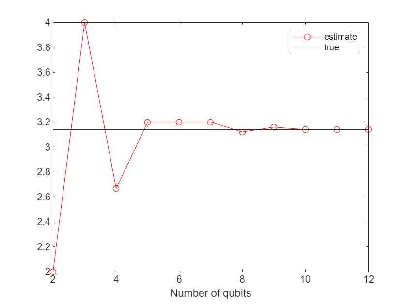
As we increase the number of qubits, we get a better approximation.
qubits = 2:12;
pies = zeros(1,length(qubits));
for n = 1:length(qubits)
pies(n) = estimatePi(qubits(n));
end
plot(qubits, pies, 'r-o')
hold on
yline(pi)
legend('estimate', 'true')
xlabel('Number of qubits')
hold off
The function can also return the circuit used in each case which allows us to visualize it. Here's the 4 qubit case
[qPi,circ] = estimatePi(4);
plot(circ)
Today I only simulated these quantum systems but you can also try running them on real quantum hardware too. How to do this using IBM's quantum services is covered in the MATLAB documentation Run Quantum Circuit on Hardware Using IBM Qiskit Runtime Services. My blog post, Quantum computing in MATLAB R2023b: On the desktop and in the cloud discusses how to run on quantum systems via AWS Braket.
So that's it from me and Guy. Whether you calculate your pi's using state of the art computing hardware or a large stone cylinder, happy pi day!


评论
要发表评论,请点击 此处 登录到您的 MathWorks 帐户或创建一个新帐户。