CLim, caxis, imshow, and imagesc
In response to "MATLAB image display - autoscaling values with imshow," MATLAB Answerer Extraordinaire ImageAnalyst posted this comment:
A discussion of the relationship and interplay of caxis(), CLim, and the values you can pass in inside the brackets to imshow() or imagesc() might be useful. For example, let's say your values range from 200 to 35,000, and you want all values less than 1000 to be blue and all values more than 29000 to be red. And you want a colorbar with 16 steps - 16 discrete colors. How would one go about that, and using which functions?
Good question! Let's have a go at it, starting with CLim.
CLim is a property of an Axes object.
To investigate CLim, start with imagesc, some elevation data, and a color bar.
load mt_monadnock.mat

imagesc(Zc)
axis image

colorbar

The Axes object controls many aspects of the plot, including the axes rulers, the ticks, the tick labels, the grid lines, and much more. The function gca ("get current axes") returns the Axes object.
ax = gca
ax =

  Axes with properties:

             XLim: [0.5000 3.0425e+03]
             YLim: [0.5000 3.0425e+03]
           XScale: 'linear'
           YScale: 'linear'
    GridLineStyle: '-'
         Position: [0.1168 0.1100 0.6965 0.8150]
            Units: 'normalized'

  Use GET to show all properties
The Axes object has a large number of properties, so by default MATLAB shows you just the most commonly used ones. If you run this code interactively, you would see a clickable "Show all properties" link.
One of those properties is CLim ("color limits"), which you can access directly this way:
ax.CLim
ans =

  141.5285  963.1366
If you look closely at the color bar in the image plot above, you can see the correspondence between it and the CLim values. ax.CLim(1) is the bottom value on the color bar, and ax.Clim(2) is the top value.
Where did those values come from, though?
They were automatically computed from the range of the data being plotted.
min(Zc(:))
ans =

  141.5285
max(Zc(:))
ans =

  963.1366
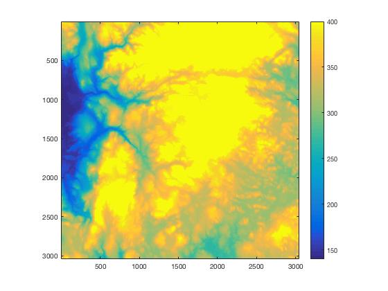
You can set the CLim yourself, though, and that changes the way the color is scaled from the data values. Let's set the color limits to expand the visible details of the lower elevations.
ax.CLim = [140 400];
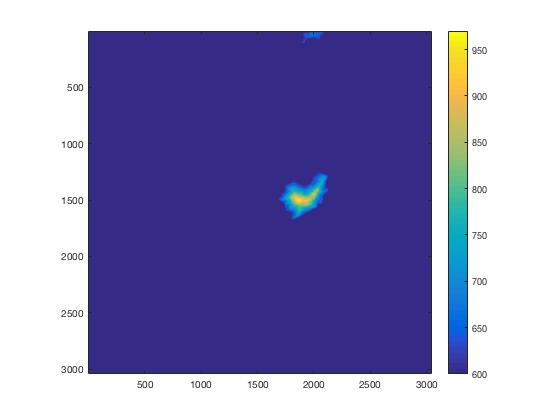
Or maybe you want to examine the upper elevations.
ax.CLim = [600 970];
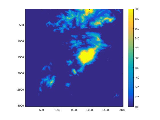
ImageAnalyst mentioned the function caxis. That's just a convenient way to set the color limits. It's one step shorter than getting the Axes using gca and then setting its CLim property.
caxis([400 600])
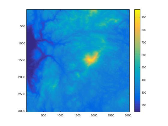
You can also use caxis to quickly get back to automatic computation of color limits.
caxis('auto')
Then ImageAnalyst asked about the [low high] syntax for imagesc and imshow. This is just another convenience for setting the color limits.
imagesc(Zc,[400 600])
axis image
colorbar

ax = gca;
ax.CLim
ans =

   400   600
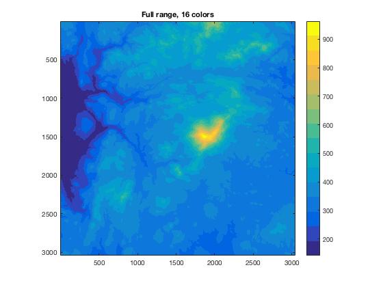
The final part of ImageAnalyst's comment concerned the number of colors. What if you only want 16 colors? Well, all of the MATLAB colormap functions take an optional input argument specifying the number of colors to use. So just call the colormap function that you want to use and pass it the desired number of colors.
caxis('auto')
colormap(parula(16))
title('Full range, 16 colors')


コメント
コメントを残すには、ここ をクリックして MathWorks アカウントにサインインするか新しい MathWorks アカウントを作成します。