
Gaussian filtering with imgaussfilt
With the R2015a release a couple of years ago, the Image Processing Toolbox added the function imgaussfilt. This function performs 2-D Gaussian filtering on images. It features a heuristic that automatically switches between a spatial-domain implementation and a frequency-domain implementation.
I wanted to check out the heuristic and see how well it works on my own computer (a 2015 MacBook Pro).
You can use imgaussfilt this way:
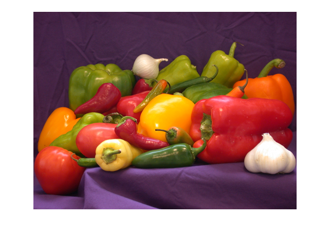
rgb = imread('peppers.png');
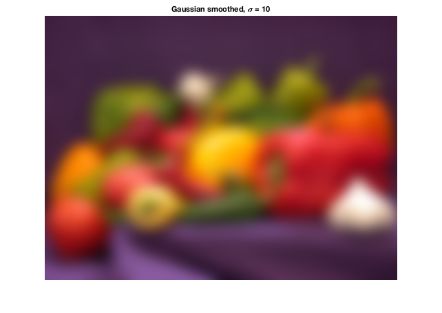
sigma = 10;
rgb_smoothed = imgaussfilt(rgb,sigma);
imshow(rgb)
imshow(rgb_smoothed)
title('Gaussian smoothed, \sigma = 10')
With this call, imgaussfilt automatically chooses between a spatial-domain or a frequency-domain implementation. But you can also tell imgaussfilt which implementation to use.
rgb_smoothed_s = imgaussfilt(rgb,sigma,'FilterDomain','spatial');
rgb_smoothed_f = imgaussfilt(rgb,sigma,'FilterDomain','frequency');
I'll use this syntax, together with the timeit function, to get rough timing curves for the two implementation methods. The heuristic used by imgaussfilt uses a few different factors to decide, including image size, Gaussian kernel size, single or double precision, and the availability of processor-specific optimizations. For my computer, with a 2000-by-2000 image array, the cross-over point is at about $\sigma = 50$. That is, imgaussfilt uses the spatial-domain method for $\sigma < 50$, and it uses a frequency-domain method for $\sigma > 50$.
Let's check that out with a set of $\sigma$ values ranging from 5 to 200.
I = rand(2000,2000);
ww = 5:5:200;
for k = 1:length(ww)
    t_s(k) = timeit(@() imgaussfilt(I,ww(k),'FilterDomain','spatial'));
end

for k = 1:length(ww)
    t_f(k) = timeit(@() imgaussfilt(I,ww(k),'FilterDomain','frequency'));
end

plot(ww,t_s)
hold on
plot(ww,t_f)
hold off
legend('spatial','frequency')
xlabel('\sigma')
ylabel('time (s)')
title('imgaussfilt - 2000x2000 image')
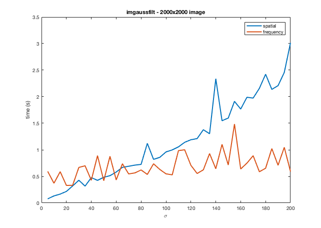
As you can see, the cross-over point of the timing curves is about the same as the threshold used by imgaussfilt. As computing hardware and optimized computation libraries evolve over time, though, the ideal cross-over point might change. The Image Processing Toolbox team will need to check this every few years and adjust the heuristic as needed.


See Also
-
Filtering fun
Blogs
-
-

评论
要发表评论,请点击 此处 登录到您的 MathWorks 帐户或创建一个新帐户。