Ka.Race.Ing-Team at Karlsruhe Institute of Technology volunteered to share in depth and hands-on their approach around vehicle controls and torque vectoring in particular. They are winners of the Simulink Student Challenge 2016. And to top it all off, Julian our guest blogger today, added two of their models on the MATLAB Central File Exchange: EV recuperation limitation, Real time derivation filter. Thanks for sharing this and the great example of community spirit!

– – –

Introduction

In recent years of electric of Formula Student, control systems have gained importance. The impact of well-tuned torque vectoring and traction control systems is comparable to a weight reduction of 10kg. However, it doesn’t come without cost to develop such a system. This introduction aims to give you an overview of where to start and to summarize your options. Developing the control system in Simulink has a lot of advantages. You do not need to be an expert programmer, it is easy to understand for others (and the poor team member who has the job in the next season). What is most important: you can use built-in MATLAB functions.

Main Processing Unit

The hardware you use can be very different. Boundary conditions for the processing unit are:

• It must be capable of the data interface, which is used in the car. In most cases that is the CAN-BUS. The computational power must be sufficient.
• There must be a possibility to compile the Simulink model for the unit.
• For telemetry, the hardware should be connected to a radio interface, for example a LAN adapter in combination with a WLAN router.

An example we are considering is the Flea3 by CarMedialab. The C2000 family by Texas Instruments is also worthy to mention. Find here a Racing Lounge blog post for an application of this type of board. Or, you can even use a Raspberry Pi for the job.

A complicated but powerful approach involved systems on a chip (SoC) involving an FPGA. Also the Racing Lounge video podcast also has addressed this topic, showing how to implement a Simulink model on a Xilinx Zynq 7000. With this hardware, you have the possibility to use a FPGA, which is relatively complicated and not necessary at least for a first attempt.

As you can see, there are a lot of possible control units, while the way of implementing your Simulink model differs depending on the hardware. For a first attempt, it can be good to use a Simulink model which directly takes the data from the CAN-BUS. Later I would recommend exporting the Simulink model with Simulink Coder and implement it in another control unit Software, which is also able to use telemetry data. This way, you can quickly change parameters without re-flashing. That saves a lot of test time.

Sensors

• Mandatory Sensors:
  • Steering angle sensor
    The most important sensor for the torque vectoring model. Steering angle is important for defining target value, such as target yaw moment (well, that is one option) but also for calculating a vehicle model.
  • Throttle pedal sensor
    This input has to be used to determine the longitudinal acceleration of the car. One has several options here: Either, it can be proportional to a sum of motor torques, factorized by a torque ratio, calculated by the torque vectoring system. Alternatively, the input is proportional to a target longitudinal acceleration as input for the torque vectoring.
  • Brake pressure sensor
    The brake pressure is needed to determine whether the motor torques work against the brakes. Then the torque must be reduced or set to zero. Therefore, it is good to know which torque is distributed from the brakes, dependent on brake pressure.
  • Electrical brake sensor
    There are two options for recuperation sensors. You can use a spring and a sensor comparable to your throttle pedal sensor. Alternatively, you can use a sensor which measures the force the driver distributes on the pedal. Most drivers prefer the second option, but it is more complicated to implement. Again, you must consider which variable is varied in your control model.
  • Motor rotational speed encoders
    These are very important for traction control and some other calculations. There is no need of extra wheel speed sensors. Taking the gear ratio into account is absolutely enough.
  • Battery voltage and battery current
    Limiting Power to 80 kW can be done by a controller. For that you need the current power. These sensors can also be interesting for different recuperation strategies.
• Optional Sensors:
  • Inertial measurement unit (IMU)
    Although not mandatory, an IMU is very important for a good control system. It contains at least an acceleration sensor and a gyroscope. Wheel loads can be calculated using accelerations. Yaw rate is a very important quantity which is calculated from the gyroscope data. For calculating an own reference speed (which doesn’t come for free in 4WD cars), it is mandatory. If you do not have the possibility to develop an IMU on your own, take an existing one and adapt a CAN interface on it, such as in that example.
  • GPS
    Not necessary for the control system if you do not want to calculate a reference speed on your own. If you want to calculate a reference speed a differential GPS (dGPS) is the better way.
  • Push- / pullrod load cell or strain gauge
    This is nice to have not only for your wheel loads in your control system, but also for other validations on your car. However, especially strain gauges are hard to implement. Normally it is also enough to calculate wheel loads using IMU data.
  • Optical speed sensor
    If you can manage to get an optical speed sensor, e.g. Kistler Correvit, for reference speed and side slip angle as a sponsoring, do not hesitate. Alternatives  are GeneSys ADMA and VBOX Speed Sensors.

Filtering and Differentiating

Most of the data you get from your sensors is noisy. For further implementations, filtering is required. Mostly, a low-pass filter is the best choice. You can decide between a finite impulse response (FIR) filter, which is a moving average, or an infinite impulse response (IIR) filter. Moving average works for us perfectly for steering angle, gyroscope data, and wheel speeds. There is no need for more advanced filters. However, make sure you take phase shift into account, which can have huge effects. Custom filters can be designed, which could look like this for a FIR filter:

FIR-Filter

Another possibility is to use low-pass filter blocks from Simulink.

Differentiating noisy signals requires more computational effort . Finite difference methods such as difference quotient or central differencing scheme (preferred) work well and almost without phase shifts. On the downside, these filters also work as high-pass filters and hence increase noise. For example, a MATLAB implementation of central differencing looks like this:

diff_central = (f-f2)/(2*dt);
% f : value to be differentiated
% f2: value of the second last time step
% dt: duration of one time step

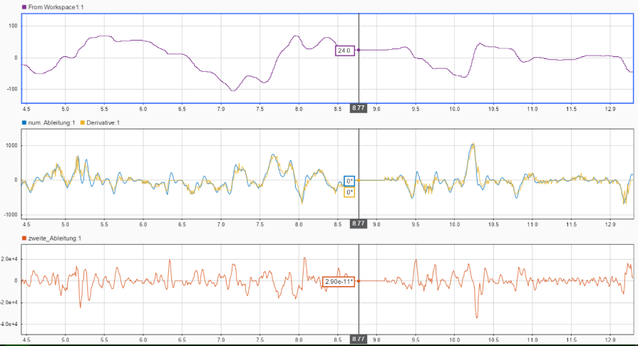
We have been using this slightly more complicated differentiating method for real time applications. For us, it works very well with small phase shifts and low noise. For steering angle, we were even able to calculate the second derivative (orange) basically without noise. You can also see the first derivative calculated with difference quotient method (yellow) and with the filter (blue). Find here a link to the model on File Exchange: Real time derivation filter.

Steering angle time signal; calculated first and second derivative

The system implements the resulting formulae of the paper. It calculates the derivatives without the use of loops. The needed inputs are the signal to derive and the duration of the (fixed) time step.

Reference Speed and Side Slip Angle

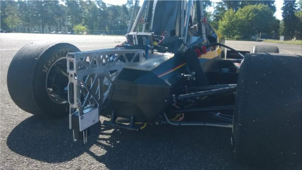
Kistler Correvit system installed on race-car

If you managed to get an optical sensor from Kistler you will not have any problems at this point.

All others must face a difficult issue. The problem is clear: A four-wheel driven car cannot take solely wheel speed data to calculate a reference speed, because all four wheels have slip. Side slip angle cannot be directly measured.

In the beginning, you may take only GPS reference speed or built up a reference speed estimator based on wheel speeds and integrated longitudinal acceleration data and assume the side slip angle to be zero. But you will notice the limits of such systems after a short time.

To manage this, some complex data fusion must be done to calculate both reference speed and side slip angle. One attempt is to use neural networks. The problem here is that you already need a lot of data with measured reference speed and side slip angle (e.g., from an optical sensor) to train the network. Furthermore, the system will differ dependent on the car, which means that you will not be able to use it every season. Another possibility is to do data fusion based on an extended Kalman filter. An introduction to Kalman filters can be found here.

The extended Kalman filter does not need measured data and can be adapted on car parameters, but it will be heavy to let it work as good as a neural network. It is very important to have a detailed update matrix, describing the whole two-dimensional vehicle dynamics. More sensors make the Kalman filter more accurate. One idea would be to take wheel speeds, IMU data and GPS position.

Validation of such systems is still heavy without being able to measure reference speed and side slip angle. So, I suggest investing some effort in getting an optical sensor.

Power Management

Another major and often underestimated topic in race-car control system design is power management.

One part of it is recuperation. The maximum recuperation torque must be limited concerning battery voltage. While the car is braking, battery voltage increases because of the internal resistance of the battery cells. When beginning to drive, the battery usually is fully charged. Hence, it is impossible to use the maximum recuperation current as the battery voltage can go above the maximum value. Therefore, you need to slightly increase recuperation power at the beginning of endurance. One way to do that is to integrate the used electrical power. Then you can multiply it with a factor and get the slightly increasing maximum of recuperation power. If the recuperation power is at recuperation current maximum, it stops to increase. Find here a link to the model on File Exchange: EV recuperation limitation -> “recup.slx”. Surprisingly, this (simple) system works very well.
Another possibility is to build up a battery model. Based on an equivalent circuit model for your cells, it is possible to predict the increase of voltage, dependent on recuperation current. This approach allows to determine which recuperation current can be used in maximum to reach exactly the maximum voltage of your cells. This video shows how to build up a battery model.

Building up a battery model is not easy, and the advantages compared to other systems is difficult to measure. However, it shows you how your battery works and there is a huge interest in design event. For both systems, I would strongly recommend implementing a controller, which hardly reduces battery current when you get over your maximum battery voltage. In our case a simple propoertional controller did the job.

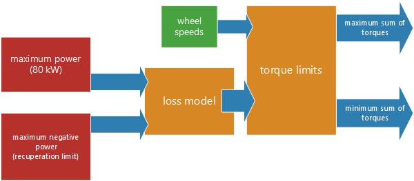
Now, you know your maximum (and maximum negative) electrical power measured by the energy meter. With a loss model of power electronics, your motors and gears, it is possible to calculate the maximum mechanical power. With the current wheel speeds (which do not differ too much between the time steps) a maximum sum of motor torques can be calculated. The torque vectoring system then distributes this sum. It is also possible to limit the torques after the torque vectoring system, while not changing the torque ratio.The choice depends on the torque vectoring.

This is a feed-forward system for the power management. The target is to get as near as possible to 80kW while not violating the rules. If you get over your maximum power with this system, it is also possible to adapt the maximum limit with a controller. Again, a simple P controller can be a first attempt.

During endurance, you will not be able to drive with 80 kW all the time. For that, the maximum power can be adapted. Most teams just set a new maximum (e.g. 50 kW) and drive through endurance with this new limit. A more advanced method is to accelerate with more power and limit it when reaching a certain speed.

Torque Vectoring

Torque vectoring makes your car fast!
Our car for example is roughly 0.4 seconds faster in skidpad with torque vectoring.
This is done in two ways: Firstly, torque vectoring can stabilize the vehicle or make it more agile. This is comparable to an ESP. Secondly, it enhances the vehicle’s grip during cornering. How this works is shown in this video.

A simple attempt, which is easy to test in the beginning, is this one: Set a constant front / rear torque distribution and calculate a left right distribution ratio on proportional to the steering angle. Even this simple system can decrease lap time significantly, when it is setup up appropriate.

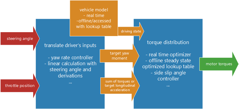
Other, more advanced, systems always have (as far as I know) a layout like this:

The driver’s inputs, which are steering angle and throttle pedal position, must be translated into variables that can be used in vehicle dynamics calculations. These are a target yaw moment and a desired longitudinal acceleration or sum of motor torques. The desired acceleration is just set proportional to the throttle pedal. Yaw moment is more complicated. An often used and well-known attempt is to apply a yaw rate controller, which sets the target yaw moment. The target yaw rate can be calculated from Ackermann geometry or optimizations on a steady state vehicle model. A yaw rate controller is especially suitable for inexperienced drivers who are not used to a vehicle swinging off. More experienced drivers sometimes feel limited when driving with a yaw rate controller. For them you can use an easier approach: just set the yaw moment proportional to steering angle and its derivative. And there are a lot more possibilities to do that. If torque distribution properly sets the yaw moment, one has a more agile or more stable car, depending on the driving situation. The task for torque distribution is to fulfill the driver’s targets, while maximizing lateral acceleration simultaneously. This calculation should be based on a double track vehicle model. Again, there are a lot of options, how to do that. The optimization can be done in real time on the vehicle, going from tire to tire and increasing its load to the maximum. Another possibility is to optimize steer angle and motor torques offline on a steady state vehicle model and put them into the Simulink model as a lookup table.
For testing of suspension and aerodynamics it should be possible to turn off torque vectoring and use the same torque on the left and right track.

Traction Control

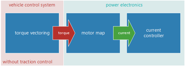
This picture shows a control system without traction control. Right after the torque vectoring system, the torques are sent from the control unit to the power electronics. When the driver pushes the throttle fully from standing, the torque vectoring sets (if there is no feedforward in torque vectoring system) motor torques to 100 percent. The power electronics will control the current given from a motor map and wheels will start to spin. That is why we need traction control.

It is still a good idea to have a switch on the steering wheel for powering off traction control. For example, if you are testing a new torque vectoring system, traction control changing torques all the time isn’t actually desired. Let your driver review your traction control with a comparison between driving with it and without it. Does it limit the torque too much?

For traction control you need to add two more systems: tire model and speed controller. The tire model is needed to calculate your target slip from the torques, this is also called an “inverse tire model”, because normally a tire model works in the other direction: from slip to force/torque. This inversion is easier to do with TMeasy than with a Pacejka model. Find here a video on tire modelling.

[VIDEO] MATLAB and Simulink Racing Lounge “MATLAB and Simulink Racing Lounge: Tire Modeling; Extracting Results from a Large Data Set“

Notice that your tire forces are highly dependent on wheel loads. Your calculation (or measurement) for that should be precise. However, if you really do not have time for building up a tire model, you can also use a linear approach between slip and force/torque.

With your current reference speed and yaw rate you can calculate your tire’s mass point velocity. By adding slip, you have calculated the target wheel speeds.

Now there are normally two possibilities. Most power electronics have an implemented speed controller. You can take that one (speed controlled), or built up another speed controller in your main control system which only begins to control, when a slip is measured, which is higher than your maximum target slip. This is called torque controlled.

At first it is easier to drive torque controlled. Real torques do not vary too much from the target torques, which means that you can be sure faults can be found in the torque vectoring system. A good reference speed is not as important as in a speed controlled system. As a speed controller, I would recommend a PI controller with some kind of anti-windup.

However, a speed controller which is not running on the power electronics will always be worse: The power electronics is directly connected to the motor’s rotational speed encoders. In this way, the controller can reach a much higher frequency and is much more precise.

There are some other problems you must consider:
Reference speed and slip can be noisy. So, your target wheel speed will be noisy too. What happens if you do not push the throttle? Most power electronics can limit their speed controller output to a certain torque, which you can send via CAN too. It is also a very good idea to use that for power limitation.
Another problem is that most of the speed controllers on power electronics are also PI controllers, which have a huge offset between target speed and measured speed, when using them in such a dynamic process like speed controlling. This means if you want to get the same torque output as in torque controlled mode, you may have to add an offset on the target speed. These offsets must be adapted such that you get out the same torque from the speed controller as it is calculated in torque vectoring when you are not driving at the tire’s maximum.

I hope you find our reasoning a little helpful.

Greetings from Karlsruhe with a very noisy “POWER FUEL!”

Best, Julian