Today’s blog is written by Neha Goel, Deep Learning Technical Evangelist on the Student Competition team at MathWorks.

Hello all! We at MathWorks, in collaboration with DrivenData, are excited to bring you this challenge. Through this challenge, you could help in finding an Alzheimer’s treatment target in reach within the next year or two. You would also get the real-world experience of working with a dataset of live videos from mouse brain. We also encourage you to use MATLAB to train your model by providing complimentary MATLAB licenses.

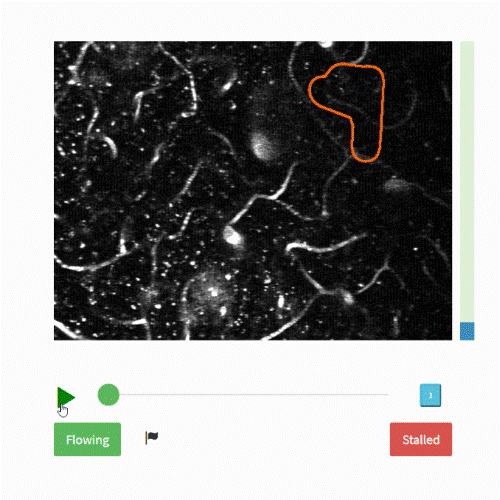
The objective of this challenge is to classify the outlined blood vessel segment as

• ‘flowing’ – if blood is moving through the vessel or
• ‘stalled’ if the vessel has no blood flow.

The main asset for solving this challenge are the videos themselves! Each video is identified by its filename, which is a numeric string followed by .mp4, e.g., 100000.mp4. All videos are hosted in a public s3 bucket.

The full training dataset contains over 580,000 videos, which is around 1.5 terabytes! To help facilitate faster model prototyping, there are two subset versions of the dataset, referred to as nano and micro.

In addition to the videos, you are provided with “train_metadata.csv” and “test_metadata.csv” files. These files consist of the information like filename, URL of each file, number of frames of each video, nano and micro subsets indication. “train_labels.csv” is the file of labels of training data.

For further details about the dataset check out the Problem Description on the competition webpage.

Getting Started with MATLAB

We are providing a basic Benchmark starter code in MATLAB on the Nanosubset version of the dataset. In this code, we walk through a basic classification model, where we are combining a pre-trained image classification model and an LSTM network. Then, we will use this model to predict the type of the vessel on test data and save a CSV file in the format required for the challenge. You can also download this MATLAB benchmark code here.

This can serve as basic code where you can start analyzing the data and work towards developing a more efficient, optimized, and accurate model using more of the training data available. Additionally, we have provided a few tips and tricks to work on the complete 1.5TB dataset. On the challenge’s Problem Description page, all required details for videos, labels performance and submission metrics are provided.

So, let’s get started with this dataset!

Load Training Data

To access the variable values from the file train_metadata.csv, load the file in the form of a tabulartext datastore in the workspace.

ttds = tabularTextDatastore("train_metadata.csv","ReadSize",'file',"TextType","string");
train =read(ttds);

We can then preview the datastore. This visualizes the first 8 rows of the file.

preview(ttds)

You can also import csv files in MATLAB using readtable function. Here, we create training labels from the train_labels.csv file and store it in a form of table. We then convert the values of the variable stalled to categorical, as most deep leaning functions used accept categorical values.

trainlabels = readtable("train_labels.csv");
trainlabels.stalled = categorical(trainlabels.stalled);

In this starter code, we will be using the nano subset of the database. Here, we retrieve the files and labels for nano subset from the tables created above and save it in variables nanotrain and nanotrainlabels. (To work with the complete dataset, you will not need this step.)

nanotrain = train(train.nano == 'True',:);
nanotrainlabels = trainlabels(train.nano == 'True',:);

Access & Process Video Files

Datastores in MATLAB are a convenient way of working with and representing collections of data that are too large to fit in memory at one time. It is an object for reading a single file or a collection of files or data. The datastore acts as a repository for data that has the same structure and formatting. To learn more about different datastores, check out the documents below:

1. Getting Started with Datastore
2. Select Datastore for File Format or Application
3. Datastores for Deep Learning

In this blog, we used the filedatastore to read each file using its URL. Each file is then processed using the readVideo helper functions, defined at the end of this blog.

We save the datastore in a MAT-file in tempdir or current folder before proceeding to next sections. If the MAT file already exists, then load the datastore from the MAT-file without reassessing them.

tempfds = fullfile(tempdir,"fds_nano.mat");

if exist(tempfds,'file')
    load(tempfds,'fds')
else

    fds = fileDatastore(nanotrain.url,'ReadFcn', @readVideo);
    files = fds.Files;

    save(tempfds,"fds");
end

Tip: For working with complete dataset (~1.5TB),create the datastore with the folder location of the training data (‘s3://drivendata-competition-clog-loss/train‘) and not with each url URL to save time and memory. This step can take a long time to run.

(Optional) We can preview the datastore and assure that each video frame is now cropped at the outlined segment.

dataOut = preview(fds);
tile = imtile(dataOut);
imshow(tile);

Classification

To create a deep learning network for video classification:

1. Convert videos to sequences of feature vectors using a pretrained convolutional neural network, such as GoogLeNet, to extract features from each frame.
2. Train an Long Short Term Memory (LSTM) network on the sequences to predict the video labels.
3. Assemble a network that classifies videos directly by combining layers from both networks.

The following diagram illustrates the network architecture.

• To input image sequences to the network, use a sequence input layer.
• To use convolutional layers to extract features, that is, to apply the convolutional operations to each frame of the videos independently, use a sequence folding layer followed by the convolutional layers.
• To restore the sequence structure and reshape the output to vector sequences, use a sequence unfolding layer and a flatten layer.
• To classify the resulting vector sequences, include the LSTM layers followed by the output layers.

Load Pretrained Convolutional Network

To convert frames of videos to feature vectors, we use the activations of a pretrained network. Load a pretrained GoogLeNet model using the googlenet function. This function requires the Deep Learning Toolbox™ Model for GoogLeNet Network support package.

netCNN = googlenet;

Convert Frames to Feature Vectors

Use the convolutional network as a feature extractor by getting the activations when inputting the video frames to the network.

This diagram illustrates the data flow through the network.

The input size should match the input size of the pretrained network, here the GoogLeNet network.  The datastore is then resized to the input size using the transform function.

inputSize = netCNN.Layers(1).InputSize(1:2);
fdsReSz = transform(fds,@(x) imresize(x,inputSize));

Convert the videos to sequences of feature vectors, where the feature vectors are the output of the activations function on the last pooling layer of the GoogLeNet network (“pool5-7x7_s1“). To analyze every size and location of the clogged vessels within the outlined segment, we do not modify the lengths of the sequences here.

Tip: After converting the videos to sequences, save the sequences in a MAT-file in the tempdir folder. If the MAT file already exists, then load the sequences from the MAT-file without reconverting them. This step can take a long time to run.

layerName = "pool5-7x7_s1";

tempFile = fullfile(tempdir,"sequences_nano.mat");

if exist(tempFile,'file')
    load(tempFile,"sequences")
else
    numFiles = numel(files);
    sequences = cell(numFiles,1);

    for i = 1:numFiles 
        fprintf("Reading file %d of %d...\n", i, numFiles); 
        sequences{i,1} = activations(netCNN,read(fdsReSz),layerName,'OutputAs','columns','ExecutionEnvironment',"auto"); 
    end

    save(tempFile,"sequences");
end

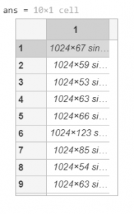
We then view the sizes of the first few sequences. Each sequence is a D-by-S array, where D is the number of features (the output size of the pooling layer) and S is the number of frames of the video.

sequences(1:10)

Prepare Training Data

Here, we prepare the data for training by partitioning the data into training and validation partitions. We assign 90% of the data to the training partition and 10% to the validation partition.

labels = nanotrainlabels.stalled;

numObservations = numel(sequences);
idx = randperm(numObservations);
N = floor(0.9 * numObservations);

idxTrain = idx(1:N);
sequencesTrain = sequences(idxTrain);
labelsTrain = labels(idxTrain);

idxValidation = idx(N+1:end);
sequencesValidation = sequences(idxValidation);
labelsValidation = labels(idxValidation);

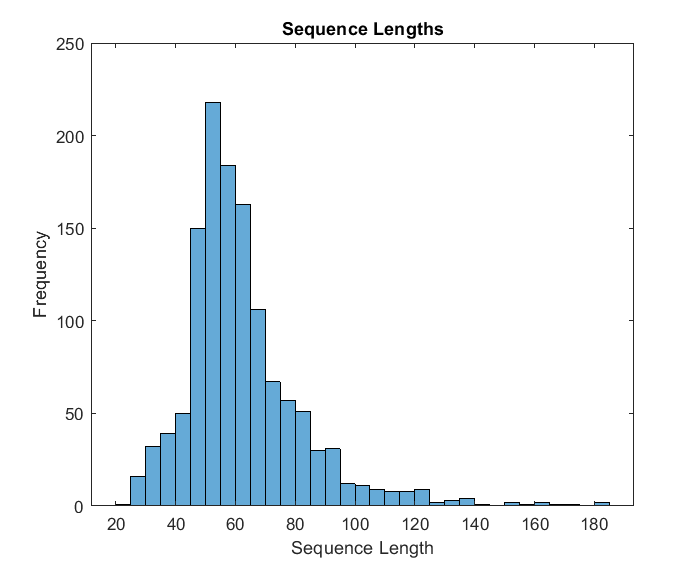
We then get the sequence lengths of the training data and visualize them in a histogram plot.

numObservationsTrain = numel(sequencesTrain);
sequenceLengths = zeros(1,numObservationsTrain);

for i = 1:numObservationsTrain
    sequence = sequencesTrain{i};
    sequenceLengths(i) = size(sequence,2);
end

figure
histogram(sequenceLengths)
title("Sequence Lengths")
xlabel("Sequence Length")
ylabel("Frequency")

Create LSTM Network

Next, create an Long Short Term Memory (LSTM) network that can classify the sequences of feature vectors representing the videos.

We then define the LSTM network architecture and specify the following network layers.

• A sequence input layer with an input size corresponding to the feature dimension of the feature vectors
• A BiLSTM layer with 2000 hidden units with a dropout layer To output only one label for each sequence by setting the ‘OutputMode‘ option of the BiLSTM layer to ‘last‘
• A fully connected layer with an output size corresponding to the number of classes, a softmax layer, and a classification layer.

numFeatures = size(sequencesTrain{1},1);
numClasses = 2;

layers = [
    sequenceInputLayer(numFeatures,'Name','sequence')
    bilstmLayer(2000,'OutputMode','last','Name','bilstm')
    dropoutLayer(0.5,'Name','drop')
    fullyConnectedLayer(numClasses,'Name','fc')
    softmaxLayer('Name','softmax')
    classificationLayer('Name','classification')];

Specify Training Options

As the next step, we specify the training options using the trainingOptions function:

• Set a mini-batch size 16, an initial learning rate of 0.0001, and a gradient threshold of 2 (to prevent the gradients from exploding).
• Truncate the sequences in each mini-batch to have the same length as the shortest sequence.
• Shuffle the data every epoch.
• Validate the network once per epoch.
• Display the training progress in a plot and suppress verbose output.

miniBatchSize = 16;
numObservations = numel(sequencesTrain);
numIterationsPerEpoch = floor(numObservations / miniBatchSize);

options = trainingOptions('adam', ...
    'MiniBatchSize',miniBatchSize, ...
    'InitialLearnRate',1e-4, ...
    'GradientThreshold',2, ...
    'Shuffle','every-epoch', ...
    'ValidationData',{sequencesValidation,labelsValidation}, ...
    'ValidationFrequency',numIterationsPerEpoch, ...
    'Plots','training-progress', ...
    'Verbose',false, ...
    'ExecutionEnvironment','auto');

Train LSTM Network

We then train the network using the trainNetwork function. Note that this function can take a long time to run due to the computations involved.

[netLSTM,info] = trainNetwork(sequencesTrain,labelsTrain,layers,options);

As the next step, we calculate the classification accuracy of the network on the validation set using classify function. You can use the same mini-batch size as you used for the training option.

YPred = classify(netLSTM,sequencesValidation,'MiniBatchSize',miniBatchSize);
YValidation = labelsValidation;
accuracy = mean(YPred == YValidation)

Assemble Video Classification Network

To create a network that classifies videos directly, assemble a network using layers from both of the created networks. Use the layers from the convolutional network to transform the videos into vector sequences and the layers from the LSTM network to classify the vector sequences.

The following diagram illustrates the network architecture.

• To input image sequences to the network, use a sequence input layer.
• To use convolutional layers to extract features, that is, to apply the convolutional operations to each frame of the videos independently, use a sequence folding layer followed by the convolutional layers.
• To restore the sequence structure and reshape the output to vector sequences, use a sequence unfolding layer and a flatten layer.
• To classify the resulting vector sequences, include the LSTM layers followed by the output layers.

Add Convolutional Layers

First, we create a layer graph of the GoogLeNet network.

cnnLayers = layerGraph(netCNN);

Then we remove the input layer (“data“) and the layers after the pooling layer used for the activations (“pool5-drop_7x7_s1“, “loss3-classifier“, “prob“, and “output“).

layerNames = ["data" "pool5-drop_7x7_s1" "loss3-classifier" "prob" "output"];
cnnLayers = removeLayers(cnnLayers,layerNames);

Add Sequence Input Layer

We create a sequence input layer that accepts image sequences containing images of the same input size as the GoogLeNet network. To normalize the images using the same average image as the GoogLeNet network, set the ‘Normalization‘ option of the sequence input layer to ‘zerocenter‘ and the ‘Mean‘ option to the average image of the input layer of GoogLeNet.

inputSize = netCNN.Layers(1).InputSize(1:2);
averageImage = netCNN.Layers(1).Mean;

inputLayer = sequenceInputLayer([inputSize 3], ...
    'Normalization','zerocenter', ...
    'Mean',averageImage, ...
    'Name','input');

We then add the sequence input layer to the layer graph. To apply the convolutional layers to the images of the sequences independently, we remove the sequence structure of the image sequences by including a sequence folding layer between the sequence input layer and the convolutional layers. We then connect the output of the sequence folding layer to the input of the first convolutional layer (“conv1-7x7_s2“).

layers = [
    inputLayer
    sequenceFoldingLayer('Name','fold')];

lgraph = addLayers(cnnLayers,layers);
lgraph = connectLayers(lgraph,"fold/out","conv1-7x7_s2");

Add LSTM Layers

The next step is to add the LSTM layers to the layer graph by removing the sequence input layer of the LSTM network. To restore the sequence structure removed by the sequence folding layer, we can include a sequence unfolding layer after the convolution layers. The LSTM layers expect sequences of vectors. To reshape the output of the sequence unfolding layer to vector sequences, we include a flatten layer after the sequence unfolding layer.

We take the layers from the LSTM network and remove the sequence input layer.

lstmLayers = netLSTM.Layers;
lstmLayers(1) = [];

Add the sequence folding layer, the flatten layer, and the LSTM layers to the layer graph. Connect the last convolutional layer (“pool5-7x7_s1“) to the input of the sequence unfolding layer (“unfold/in“).

layers = [
    sequenceUnfoldingLayer('Name','unfold')
    flattenLayer('Name','flatten')
    lstmLayers];

lgraph = addLayers(lgraph,layers);
lgraph = connectLayers(lgraph,"pool5-7x7_s1","unfold/in");

To enable the unfolding layer to restore the sequence structure, connect the “miniBatchSize” output of the sequence folding layer to the corresponding input of the sequence unfolding layer.

lgraph = connectLayers(lgraph,"fold/miniBatchSize","unfold/miniBatchSize");

Assemble Network

We then check that the network  is valid using the analyzeNetwork function.

analyzeNetwork(lgraph)

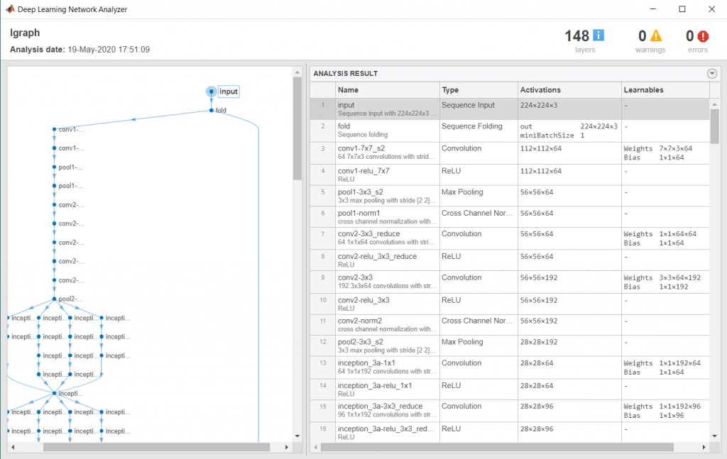
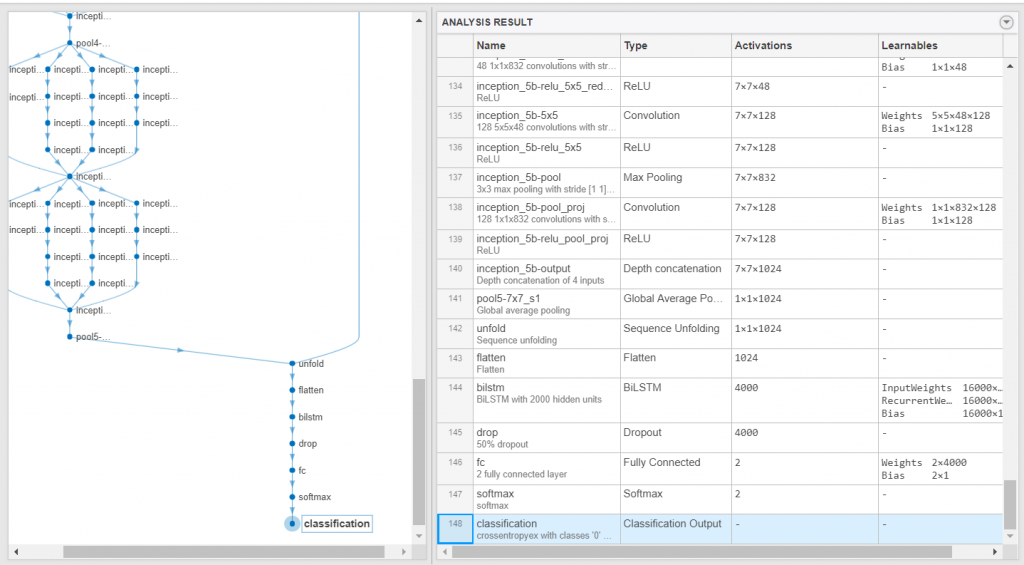
And, assemble the network so that it is ready for prediction using the assembleNetwork function.

net = assembleNetwork(lgraph)

Prepare Test Data

Just as we did with the training data, we will now read the test files in a filedatastore and crop the frames using the readVideo function. The cropped files datastore is then resized as per the inputSize using the transform function.

When we use all the files from a folder, we can directly give the s3 folder url while creating the datastore. This speed up the creation of the datastore. 

testfds = fileDatastore('s3://drivendata-competition-clog-loss/test/','ReadFcn', @readVideo);
testfdsReSz = transform(testfds,@(x) {imresize(x,inputSize)});

Classify Using Test Data

Once we have our trained network, we can perform predictions on our test set. To do so, we classify the test set videos using the assembled network. The classify function expects a cell array containing the input videos, so you must input a 1-by-1 cell array containing the video.

testFiles = testfds.Files;
numTestFiles = numel(testFiles);

YPred = cell(numTestFiles,1);

for i = 1:numTestFiles
    fprintf("Reading file %d of %d...\n", i, numTestFiles);
    YPred{i,1} = classify(net,read(testfdsReSz),'ExecutionEnvironment','auto');
end

Save Submission to File

We create a table of the results based on the filenames and prediction scores. The desired file format for submission is a csv file with coulmn names: filename and stalled.

We will place all the test results in a MATLAB table, which makes it easy to visualize and to write to the desired file format.

test = readtable("test_metadata.csv");
testResults = table(test.filename,YPred(:,1),'VariableNames',{'filename','stalled'});

We then write the results to a CSV file. This is the file you will submit for the challenge.

writetable(testResults,'testResults.csv');

Helper Functions

The readVideofunction reads the video in filename and returns a cropped 4-D frame.

The area of interest in the entire video is the orange colored area in each frame of the video which we would want to extract to use for the rest of our training. Hence, each frame is cropped as per the bounding box of the segment, calculated using the detectROI function.

function video = readVideo(filename)

vr = VideoReader(filename);
i = 0;
% video = zeros;

while hasFrame(vr)
    i = i+1;
    frame = readFrame(vr);
    if i < 2
        Bbox = detectROI(frame);
    end
    frame = imcrop(frame, Bbox);
    video(:,:,:,i)=frame;
end

end

The detectROIfunction detects the outlined segment and thresholds the image based on threshold values defined. This function is generated using MATLAB’s color thresholder app. For detecting the area specified by the orange colured markers, we used Blob Analysis. We chose to keep the area of interest as the blob with the largest major axis. Check out the following videos to learn more.

• How to Segment Images Using Color Thresholding
• Object Detection using Blob analysis

function [Bbox] = detectROI(frameIn)

%% Setup the detector and initialize variables
persistent detector
if isempty(detector)
    detector = vision.BlobAnalysis('BoundingBoxOutputPort',true,'MajorAxisLengthOutputPort',true);
end

threshold = [104 255; 13 143; 9 98];

mask = (frameIn (:,:,1) >= threshold(1,1))& (frameIn (:,:,1) <= threshold(1,2))&...
(frameIn (:,:,2) >= threshold(2,1))& (frameIn (:,:,2) <= threshold(2,2))&...
(frameIn (:,:,3) >= threshold(3,1))& (frameIn (:,:,3) <= threshold(3,2));

[~, ~, Bbox1, majorAxis] = detector(mask);

if ~isempty(majorAxis)
% Identify Largest Blob
    [~,mIdx] = max(majorAxis);
    Bbox = Bbox1(mIdx,:);

end

end

Thanks for following along with this blog. We are excited to find out how you will modify this starter code and make it yours. We strongly recommend looking at our Deep Learning Tips & Tricks page for more ideas on how you can improve the benchmark model. You can also check out this blog: Are you ready for a Video Classification Challenge, to learn 5 different methods for Video Classification.

Feel free to reach out to us in the DrivenData forum if you have any further questions.