
Game of Life, Part 1, The Rule
This is part one of a series of posts about John Conway's Game of Life. One deceptively simple rule leads to an incredible variety of patterns, puzzles, and unsolved mathematical problems, and a beautiful use of MATLAB sparse matrices.
The fascination of Conway's Game of Life is that this deceptively simple rule leads to an incredible variety of patterns, puzzles, and unsolved mathematical problems -- just like real life.
 Our first population starts with live cells in an L-shape. All three cells have two live neighbors, so they survive. The dead cell that they all touch has three live neighbors, so it springs to life. None of the other dead cells have enough live neighbors to come to life. So the result, after one step, is the stationary four-cell population known as the block. Each of the live cells has three live neighbors and so lives on. None of the other cells can come to life. The four-cell block lives forever.
 The other three-cell initial population is I-shaped. The two possible orientations are shown in the two steps of the blinker. At each step, two end cells die, the middle cell stays alive, and two new cells are born to give the orientation shown in the other step. If nothing disturbs it, this three-cell blinker keeps blinking forever. It repeats itself in two steps; this is known as its period.
 Four steps in the evolution of one of the most interesting five-cell initial populations, the glider, are shown here. At each step two cells die and two new ones are born. After four steps the original population reappears, but it has moved diagonally down and across the grid. It moves in this direction forever, continuing to exist in the infinite universe.
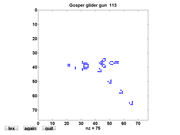 Bill Gosper developed his Glider Gun at MIT in 1970. The portion of the population between the two static blocks oscillates back and forth. Every 30 steps, a glider emerges. The result is an infinite stream of gliders that fly off into the expanding universe. This was the first example discovered of a finite starting population whose growth is unbounded.
Here is a movie, Gosper Glider Gun Movie, that captures every fifth step for 140 steps. The first glider just reaches the edge of the frame and life_lex is about the resize its view when I stop the recording. You will have to download the code and run it yourself to see how the resizing works.
Bill Gosper developed his Glider Gun at MIT in 1970. The portion of the population between the two static blocks oscillates back and forth. Every 30 steps, a glider emerges. The result is an infinite stream of gliders that fly off into the expanding universe. This was the first example discovered of a finite starting population whose growth is unbounded.
Here is a movie, Gosper Glider Gun Movie, that captures every fifth step for 140 steps. The first glider just reaches the edge of the frame and life_lex is about the resize its view when I stop the recording. You will have to download the code and run it yourself to see how the resizing works.
Contents
The Rule
The "Game of Life" was invented by John Horton Conway, a British-born mathematician who is now a professor at Princeton. The game made its public debut in the October 1970 issue of Scientific American, in the Mathematical Games column written by Martin Gardner. At the time, Gardner wroteThis month we consider Conway's latest brainchild, a fantastic solitaire pastime he calls "life". Because of its analogies with the rise, fall and alternations of a society of living organisms, it belongs to a growing class of what are called "simulation games"--games that resemble real-life processes. To play life you must have a fairly large checkerboard and a plentiful supply of flat counters of two colors.
Today Conway's creation is known as a cellular automaton and we can run the simulations on our computers instead of checkerboards. The universe is an infinite, two-dimensional rectangular grid. The population is a collection of grid cells that are marked as alive. The population evolves at discrete time steps known as generations. At each step, the fate of each cell is determined by the vitality of its eight nearest neighbors and this rule:- A live cell with two live neighbors, or any cell with three live neighbors, is alive at the next step.
Block
If the initial population consists of three live cells then, because of rotational and reflexive symmetries, there are only two different possibilities; the population is either L-shaped or I-shaped.
Our first population starts with live cells in an L-shape. All three cells have two live neighbors, so they survive. The dead cell that they all touch has three live neighbors, so it springs to life. None of the other dead cells have enough live neighbors to come to life. So the result, after one step, is the stationary four-cell population known as the block. Each of the live cells has three live neighbors and so lives on. None of the other cells can come to life. The four-cell block lives forever.
Blinker
The other three-cell initial population is I-shaped. The two possible orientations are shown in the two steps of the blinker. At each step, two end cells die, the middle cell stays alive, and two new cells are born to give the orientation shown in the other step. If nothing disturbs it, this three-cell blinker keeps blinking forever. It repeats itself in two steps; this is known as its period.
Glider
Four steps in the evolution of one of the most interesting five-cell initial populations, the glider, are shown here. At each step two cells die and two new ones are born. After four steps the original population reappears, but it has moved diagonally down and across the grid. It moves in this direction forever, continuing to exist in the infinite universe.
Infinite Universe
So how, exactly, does an infinite universe work? The same question is being asked by astrophysicists and cosmologists about our own universe. Over the years, I have offered three different MATLAB Game of Life programs that have tackled this question three different ways. The MATLAB /toolbox/matlab/demos/ directory contains a program life that Ned Gulley and I wrote 20 years ago. This program uses toroidal boundary conditions and random starting populations. These are easy to implement, but I have to say now that they do not provide particularly satisfactory Game of Life simulations. With toroidal boundary conditions cells that reach an edge on one side reenter the universe on the opposite side. So the universe isn't really infinite. And the random starting populations are unlikely to generate the rich configurations that make Life so interesting. A few years ago, I published the book Experiments with MATLAB that includes a chapter on Game of Life and a program lifex. The program reallocates storage in the sparse data structure as necessary to accommodate expanding populations and thereby simulates an infinite universe. The viewing window remains finite, so the outer portions of the expanding populating leave the field of view. The starting populations for lifex are obtained from the Life Lexicon, a valuable resource cataloging several hundred terms related to the Game of Life. Life Lexicon includes over four hundred interesting starting populations. You can also visit a graphic version of the Lexicon. My latest program, which I am describing in this and later posts of this blog, uses the same dynamic storage allocation as lifex. But it features an expanding viewing window, so the entire population is always in sight. The individual cells get smaller as the view point recedes. The program also accesses Life Lexicon, so I've named it life_lex. It is now available from the MATLAB Central File Exchange; see the submission Game of Life. The static screen shot and the movies in this post are from life_lex.Full Screen Video Playback
I had hoped to capture the output from life_lex in such a way that you could play it back at a reasonable resolution and frame rate. But that involves video codecs and YouTube intellectual property agreements and all kinds of other stuff that I did not want to get involved in for this week's blog. Maybe later. It is easy to insert half a dozen lines of code into a MATLAB program to produce animated GIF files -- an ancient technology that is good enough for our purposes today. But it is not practical to capture every step. The resulting .gif files are too large and the playback is too slow. However the following two examples show it is possible to produce acceptable movies by not recording every frame.Glider Gun
Bill Gosper developed his Glider Gun at MIT in 1970. The portion of the population between the two static blocks oscillates back and forth. Every 30 steps, a glider emerges. The result is an infinite stream of gliders that fly off into the expanding universe. This was the first example discovered of a finite starting population whose growth is unbounded.
Here is a movie, Gosper Glider Gun Movie, that captures every fifth step for 140 steps. The first glider just reaches the edge of the frame and life_lex is about the resize its view when I stop the recording. You will have to download the code and run it yourself to see how the resizing works.
Noah's Ark
I think this is an amazing evolution. The Lexicon saysThe name comes from the variety of objects it leaves behind: blocks, blinkers, beehives, loaves, gliders, ships, boats, long boats, beacons and block on tables.
We've learned about a few of these things -- blocks, blinkers, and gliders. But what are the others? Welcome to the world of the Game of Life. For this movie I've captured every 50th step of 2000 steps. You can see why the expanding universe and the life_lex resizing are necessary, Noah's Ark Movie.- 类别:
- Matrices


评论
要发表评论,请点击 此处 登录到您的 MathWorks 帐户或创建一个新帐户。