A look at the structure, and the eigenvalues and singular values of interesting test matrices.

Contents

Wilkinson

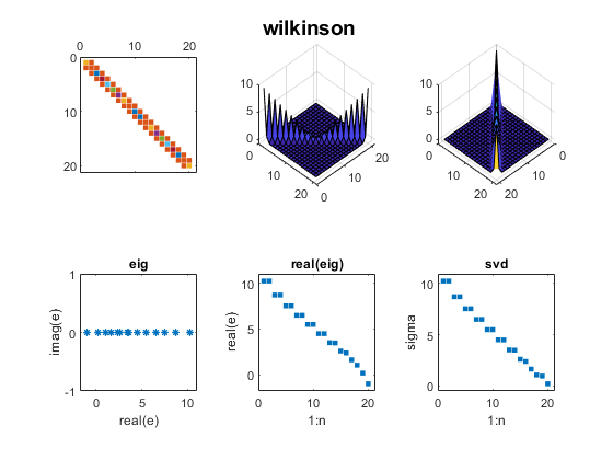
J. H. Wilkinson's most famous examples are Wn+, a family of symmetric, tridiagonal matrices with pairs of "remarkably" and "pathologically" close eigenvalues. The two largest eigenvalues of W20+,

   10.246194182902979 and
   10.246194182903745,

agree to 12 decimal places.

For more, see my blog post on Wilkinson matrices. And see page 308 of Wilkinson's The Algebraic Eigenvalue Problem.

    n = 20;
    m = (n-1)/2;
    D = diag(ones(n-1,1),1);
    A = diag(abs(-m:m)) + D + D';
    mat_expo(A,'wilkinson')

Parter

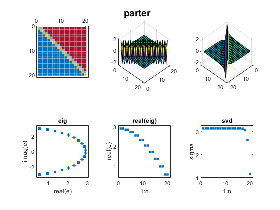
One of my favorite test matrices is this nonsymmetric cousin of the Hilbert matrix. I was surprised when I discovered that most of its singular values are equal to pi. Seymour Parter explained why. See Surprising SVD, Square Waves and Pi.

    j = 1:n;
    k = j';
    A = 1./(k-j+1/2);
    mat_expo(A,'parter')

Bucky

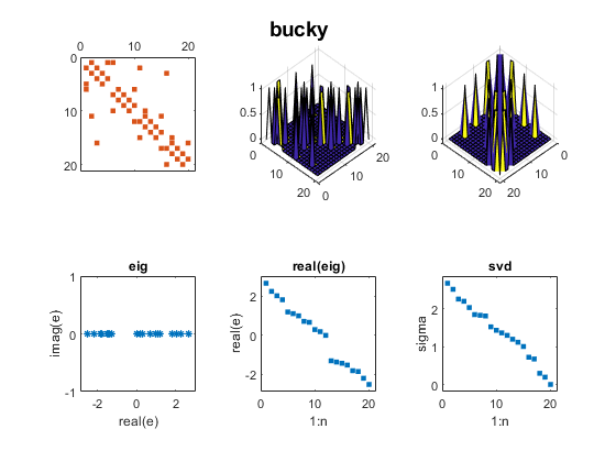
The leading 20-by-20 submatrix of the 60-by-60 Bucky Ball is symmetric, so its eigenvalues are real. But the matrix is not positive definite, so the eigenvalues do not equal the singular values. See Bringing Back the Bucky Ball.

    B = bucky;
    A = B(1:n,1:n);
    mat_expo(A,'bucky')
    

Checkerboard

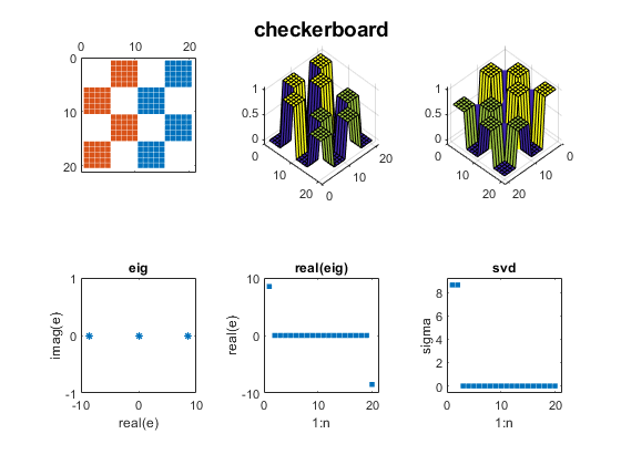
We introduced the Checkerboard family just two weeks ago; see Two Flavors of SVD. There are only two nonzero eigenvalues and singular values.

    A = checkerboard(n/4,2,2);
    mat_expo(A,'checkerboard')

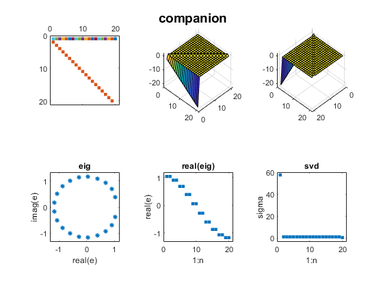
Companion

Before 1965, the fact that the eigenvalues of a companion matrix are equal to the zeros of the polynomial with coefficients in the first row was often the basis of methods to compute matrix eigenvalues. But the discovery of modern QR methods allowed the first MATLAB to reverse this approach and compute polynomial zeros as matrix eigenvalues.

In this example, the polynomial coefficients are 1:n+1 and the polynomial zeros lie on a nearly circular curve in the complex plane.

    c = 2:n+1;
    A = diag(ones(n-1,1),-1);
    A(1,:) = -c;
    mat_expo(A,'companion')

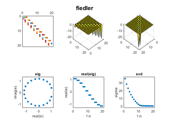
Fiedler

Fiedler companion matrix. Discovered by a contemporary Czech mathematician, Miroslav Fiedler, this matrix distributes the polynomial coefficients along the diagonals of an elegant pentadiagonal matrix whose eigenvalues are equal to the zeros of the polynomial. See Fiedler companion matrix.

Here is the same polynomial as the traditional companion matrix.

    A = fiedler(c);
    mat_expo(A,'fiedler')
    

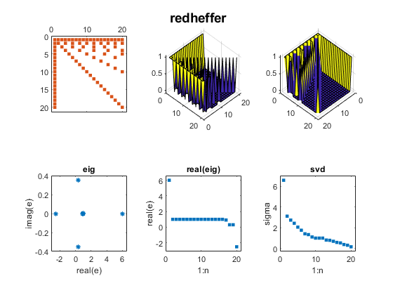
Redheffer

The Redheffer matrix has been in the gallery for a long time, but I ignored it until last September. Then I began a long series of blog posts. See Redheffer and One Million Dollars and Möbius, Mertens and Redheffer.

Most of the eigenvalues of the Redheffer matrix are equal to one. The product of all the eigenvalues, the determinant, is the Mertens function, which is related to the Riemann hypothesis.

    A = gallery('redheff',n);
    mat_expo(A,'redheffer')

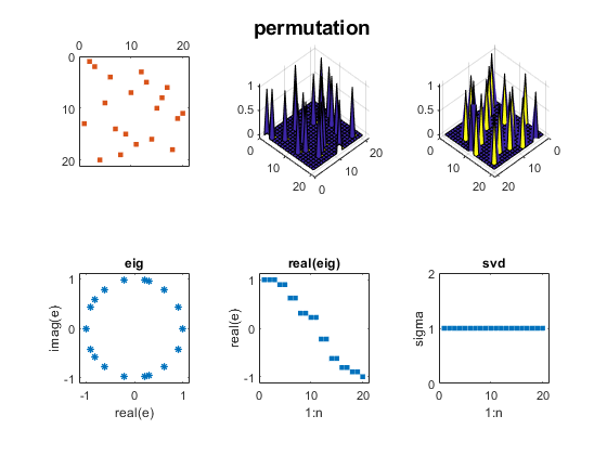
Permutation

A permutation matrix has a single 1 in each row and column and 0's elsewhere. The matrix is orthogonal, so all the eigenvalues lie on the unit circle and all the singular values are equal to one.

    p = randperm(n);
    A = sparse(p,1:n,1);
    mat_expo(A,'permutation')
    

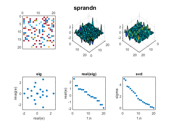
Random

This random matrix has about 1/3 of its elements equal to zero and the remaining elements normally distributed about zero. I have included such a matrix in this exposition to represent matrices in general that do not have particularly remarkable eigenvalues and singular values.

    A = sprandn(n,n,1/3);
    mat_expo(A,'sprandn')
            

Software

You can publish the source for this blog post if you also have the three functions in Mat_Expo_mzip.

Get the MATLAB code

Published with MATLAB® R2024b