
Newton’s Method Fractals
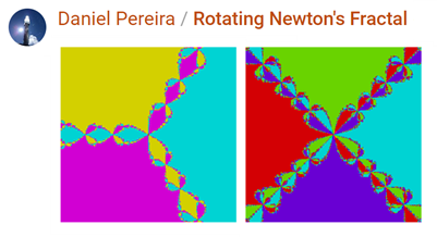
Recently I've seen a number of fractal images created with Newton's method. For instance, Daniel Pereira had two spectacular animations in the recent Flipbook Mini-Hack contest.
Here's another example of the kind of picture I'm talking about.

How is such an image made? What does it represent? It's one of those things where complexity is hiding behind something that, on its face, seems straightforward.
To motivate this, consider this question: How do you find the roots of this polynomial?
x3 - 2·x2 - 11·x + 12.
That is, for what values of x is this equation true? x3 - 2·x2 - 11·x + 12 = 0
There are a number of ways to answer this question. If you’re good at factoring polynomials, you might recognize that this is (x-4)(x-1)(x+3). Another answer is to use a little MATLAB magic. MATLAB represents polynomials as vectors containing the coefficients ordered by descending powers. Here is that same polynomial in vector form.
>> p = [1 -2 -11 12]
Once in the right form, there’s a command ROOTS that will answer our question directly.
>> roots(p)
ans =
  -3.0000
   4.0000
   1.0000
But let's say that your polynomial won't factor so easily, and you don't have a computer handy. Let’s imagine you're Isaac Newton and you want to find the roots of this polynomial. Now what?
As it happens, Newton is credited with a nifty iterative method for finding the roots in a situation like this. You start with a guess, and you use the slope of the curve at that point to make a better guess. Keep repeating this process until you get as close as you want to zero.
Let's start with a guess at -1.9.

x=-1.9000, f(x)=18.8210
x=-4.4331, f(x)=-65.6622
x=-3.4335, f(x)=-14.2877
x=-3.0585, f(x)=-1.6770
x=-3.0013, f(x)=-0.0364
x=-3.0000, f(x)=-0.0000
If we start at -1.9, we end up finding the root at -3 in around six iterations. But wait! There are three roots to this polynomial. It turns out that different starting locations will converge to different roots. So for every starting guess, there is a corresponding root. This is where things get interesting.
This iterative process maps an initial guess to a root. You can think of the resulting map as being divided into basins. Different basins drain into different roots. We can color these basins according to the root to which that starting point will eventually converge. Additionally, we'll keep track of how many iterations it takes to converge (that is, to reach the same tolerance). The curve in the top graph is colored according its corresponding root. Each colored region represents a different basin.

Curiously, these basins aren't always well defined. As we zoom into the boundaries between two basins, we keep finding smaller and smaller regions that converge to different roots. This back-and-forth convergence continues no matter how much you zoom in. This phenomenon is sometimes called a fractal basin boundary.
Now that we've demonstrated this for the real number line, you may wonder: can we generalize to the complex plane? Yes we can, because MATLAB is awesome! Since complex numbers are a native data type, you can use exactly the same code as in the one dimensional case.
So let's examine a more complicated polynomial. This one has complex roots. We'll use the process shown above to find the root basins on the complex plane.
What are the roots of this polynomial?
8·x7 + x6 + 3·x5 + 7·x4 + 2·x3 + 4·x2 + 5·x + 6
Since it is a seventh order polynomial, there are seven roots to this equation. Every point on the complex plane maps to one of them. So every single pixel in this plot is the result of Newton's method. But the borders between these regions are demented fractals.

Look how simple the code is! There's only one line right in the middle that's doing all the heavy lifting.
p = [8 1 3 7 2 4 5 6];

% Make anonymous functions for the polynomial and its derivative.
f  = @(x) polyval(p,x);
df = @(x) polyval(polyder(p),x);

span = linspace(-1.5,1.5,300);
[x,y] = meshgrid(span,span);
z = x + 1i*y;

% Apply Newton's method
for k = 1:50
  z = z - f(z)./df(z);
end

% Use ANGLE as a proxy to display the root
imagesc(span,span,angle(z))
axis square

% Show the roots
hold on
plot(roots(p), ...
  LineStyle="none", ...
  Marker="pentagram", ...
  MarkerFaceColor="red", ...
  MarkerSize=18)
hold off
And how many iterations did it take at each point to converge to that root? That's the picture we started with at the top of the post.
Now that you know the basics, it’s easy to make some eye-popping animations. Here's one of my own additions to the recent Flipbook contest.

If you want to learn more, take a look at Cleve's post on this topic: Fractal Global Behavior of Newton’s Method.


コメント
コメントを残すには、ここ をクリックして MathWorks アカウントにサインインするか新しい MathWorks アカウントを作成します。